Author Samuel Hangouët
Category Program Analysis
Tags machine learning, function similarity, data analysis, binary analysis, GNN, tool, graph neural networks, 2026
pcode_graph is a Python library, published by Quarkslab, suitable to build semantic graphs from binary code. We present how to use it to detect function similarities in binaries.
Context
We introduce here the Python library pcode_graph, a tool developed at Quarkslab to abstract the semantics of binary code. It provides an API to build and visualize Control & Data flow Graphs (CDG) from a function, a basic-block or any arbitrary piece of code.
As soon as you start looking into the automated analysis of binaries, you quickly realize that many use cases require extracting a semantic representation of a piece of code. For example, such a representation could be used to:
- Identify the type(s) of obfuscation applied;
- Build a database of gadgets or automatically chain them to do ROP;
- Find changes between two successive versions of the same binary;
- Look for a function in a database of binaries;
- Look for vulnerabilities;
- Deobfuscate a piece of binary.
This last use case was the subject of a research paper published at ESANN 2026 using the pcode_graph library, but it was not open-sourced at the time of publication.
To present the library, here we are going to focus on the detection of similarities between functions. More precisely, we will train a neural network to recognize a function, independently of the architecture, the compiler and the options used to compile it. For that, we will use the Cisco-Talos dataset.
The library is available from Quarkslab's pcode_graph repository on GitHub. It can also be installed directly with pip:
(venv) $ pip install pcode_graph
Extracting a semantic graph
Many methods exist to teach a model to compare two binary functions.
A basic approach is to extract statistical features such as the number of instructions, the number of basic blocks, the mnemonic frequencies, etc. This yields a table of features on which the learning is performed. This can be good enough to perform some basic tasks, like malware classification.
jTrans feeds the assembly (with a bit of preprocessing) into a language-processing model.
From a production perspective, several tools were compared prior to creating Quarkslab's Sighthouse tool.
Here we are going to extract a semantic graph, a representation of what the piece of code does disregarding how it does it, for example the specific CPU instructions. Note that this is not necessarily the most relevant approach: the choice depends entirely on your use case and your data.
Let's take a very simple piece of code:
int do_it(int a, int b)
{
    if (a == b)
        return a + b;
    return 0;
}
and compile it so as to get a small piece of assembly:
clang test.c -o test.o -Oz -c
On x86_64 we get:
lea   ecx, [rsi + rdi*0x1]
xor   eax, eax
cmp   edi, esi
cmovz eax, ecx
ret
Now let's try to compile it without optimization:
push rbp
mov  rbp, rsp
mov  dword ptr [rbp + -0x8], edi
mov  dword ptr [rbp + -0xc], esi
mov  eax, dword ptr [rbp + -0x8]
cmp  eax, dword ptr [rbp + -0xc]
jnz  0x1d
mov  eax, dword ptr [rbp + -0x8]
add  eax, dword ptr [rbp + -0xc]
mov  dword ptr [rbp + -0x4], eax
jmp  0x24
mov  dword ptr [rbp + -0x4], 0x0
mov  eax, dword ptr [rbp + -0x4]
pop  rbp
ret
These are two versions of the same function compiled with the same compiler for the same architecture, and yet:
- The second version is three times longer.
- The only mnemonic they have in common is CMP, and it works on different operands.
- The second one has three basic blocks against a single one for the first.
These points highlight the limits of statistical feature extraction for function comparison.
Let's now look at the optimized version. If we swap the two first instructions, the semantics remain unchanged:
xor   eax, eax
lea   ecx, [rsi + rdi*0x1]
cmp   edi, esi
cmovz eax, ecx
ret
While the order of instructions can be of interest to detect the compiler used, for our use case we are to the contrary looking for a representation that is ideally identical for identical code semantics, otherwise our model would have to learn to ignore all the semantically equivalent permutations of a same function.
To do so, we are going to extract the data flow graph of the function.
In order to abstract away the architecture, we use the pypcode library, a binding of SLEIGH which translates binary code into Ghidra's low-level internal representation. One benefit of P-Code is that it is limited to 63 distinct opcodes (at the Raw level, excluding IMARK). Compared to the thousands of x86_64 mnemonics, this limits the possibilities of expressing the same semantics in different ways. It is also a representation that makes building a data flow graph easier.
We can directly use the pcode_graph CLI to get the P-Code:
cdg pcode test.o > test.pcode
We get the following file:
imark [0x0]
$37632 = int_mult RDI, #0x1
$38144 = int_add RSI, $37632
ECX = subpiece $38144, #0x0
RCX = int_zext ECX
imark [0x3]
CF = #0x0
OF = #0x0
EAX = int_xor EAX, EAX
RAX = int_zext EAX
SF = int_sless EAX, #0x0
ZF = int_equal EAX, #0x0
$361216 = int_and EAX, #0xff
$361472 = popcount $361216
$361728 = int_and $361472, #0x1
PF = int_equal $361728, #0x0
imark [0x5]
$515328 = EDI
CF = int_less $515328, ESI
OF = int_sborrow $515328, ESI
$515840 = int_sub $515328, ESI
SF = int_sless $515840, #0x0
ZF = int_equal $515840, #0x0
$361216 = int_and $515840, #0xff
$361472 = popcount $361216
$361728 = int_and $361472, #0x1
PF = int_equal $361728, #0x0
imark [0x7]
$505344 = ECX
RAX = int_zext EAX
$505600 = bool_negate ZF
cbranch [0xa], $505600
EAX = $505344
imark [0xa]
RIP = load #0x6b970f0, RSP
RSP = int_add RSP, #0x8
return RIP
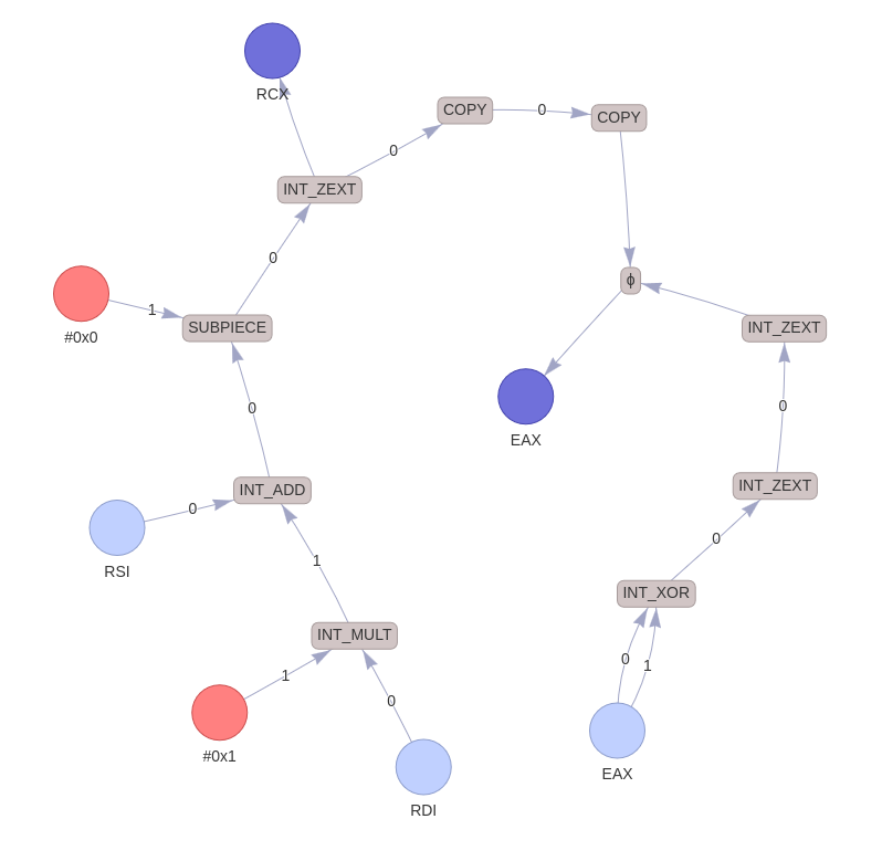
Ok, that's fairly verbose... To break instructions down into basic operations, pypcode introduces many temporary variables. But there is nothing to worry about: these variables will subsequently be ignored and will only make up edges of our data flow graph.
Before building the graph, we start by applying several analysis passes to the P-Code:
- Instruction indexing (to resolve jumps);
- Unreachable code detection;
- Data flow analysis.
These results can be displayed as a table in markdown format:
cdg table test.o
| index | op | preds | succs | input defs | reachable | exit def |
|---|---|---|---|---|---|---|
| 0 | imark [0x0] | entry | 1 | x | ||
| 1 | $37632 = int_mult RDI, #0x1 | 0 | 2 | RDI from entry | x | |
| 2 | $38144 = int_add RSI, $37632 | 1 | 3 | RSI from entry, $37632 from 1 | x | |
| 3 | ECX = subpiece $38144, #0x0 | 2 | 4 | $38144 from 2 | x | |
| 4 | RCX = int_zext ECX | 3 | 5 | ECX from 3 | x | RCX |
| 5 | imark [0x3] | 4 | 6 | x | ||
| 6 | CF = #0x0 | 5 | 7 | x | ||
| 7 | OF = #0x0 | 6 | 8 | x | ||
| 8 | EAX = int_xor EAX, EAX | 7 | 9 | EAX from entry, EAX from entry | x | |
| 9 | RAX = int_zext EAX | 8 | 10 | EAX from 8 | x | |
| 10 | SF = int_sless EAX, #0x0 | 9 | 11 | EAX from 9 | x | |
| 11 | ZF = int_equal EAX, #0x0 | 10 | 12 | EAX from 9 | x | |
| 12 | $361216 = int_and EAX, #0xff | 11 | 13 | EAX from 9 | x | |
| 13 | $361472 = popcount $361216 | 12 | 14 | $361216 from 12 | x | |
| 14 | $361728 = int_and $361472, #0x1 | 13 | 15 | $361472 from 13 | x | |
| 15 | PF = int_equal $361728, #0x0 | 14 | 16 | $361728 from 14 | x | |
| 16 | imark [0x5] | 15 | 17 | x | ||
| 17 | $515328 = EDI | 16 | 18 | EDI from entry | x | |
| 18 | CF = int_less $515328, ESI | 17 | 19 | $515328 from 17, ESI from entry | x | CF |
| 19 | OF = int_sborrow $515328, ESI | 18 | 20 | $515328 from 17, ESI from entry | x | OF |
| 20 | $515840 = int_sub $515328, ESI | 19 | 21 | $515328 from 17, ESI from entry | x | |
| 21 | SF = int_sless $515840, #0x0 | 20 | 22 | $515840 from 20 | x | SF |
| 22 | ZF = int_equal $515840, #0x0 | 21 | 23 | $515840 from 20 | x | ZF |
| 23 | $361216 = int_and $515840, #0xff | 22 | 24 | $515840 from 20 | x | |
| 24 | $361472 = popcount $361216 | 23 | 25 | $361216 from 23 | x | |
| 25 | $361728 = int_and $361472, #0x1 | 24 | 26 | $361472 from 24 | x | |
| 26 | PF = int_equal $361728, #0x0 | 25 | 27 | $361728 from 25 | x | PF |
| 27 | imark [0x7] | 26 | 28 | x | ||
| 28 | $505344 = ECX | 27 | 29 | ECX from 4 | x | |
| 29 | RAX = int_zext EAX | 28 | 30 | EAX from 9 | x | EAX |
| 30 | $505600 = bool_negate ZF | 29 | 31 | ZF from 22 | x | |
| 31 | cbranch [0xa], $505600 | 30 | 33, 32 | $505600 from 30 | x | |
| 32 | EAX = $505344 | 31 | 33 | $505344 from 28 | x | EAX |
| 33 | imark [0xa] | 32, 31 | 34 | x | ||
| 34 | RIP = load #0x33fd1630, RSP | 33 | 35 | MEMORY from entry, RSP from entry | x | RIP |
| 35 | RSP = int_add RSP, #0x8 | 34 | 36 | RSP from entry | x | RSP |
| 36 | return RIP | 35 | elsewhere | RIP from 34 | x |
Since pcode_graph was initially designed to work on small chunks of code, the CFG is built directly at the level of the P-Code operations instead of extracting basic-blocks. Beware that this could change in the near future.
From these elements the dataflow graph is easy to build:
Then, a simplification pass removes nodes that are useless or that carry information which can otherwise be found implicitly in the graph:
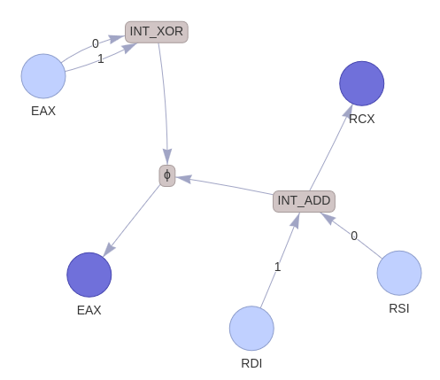
To generate this representation as an HTML file (via pyvis), you can use the cdg tool provided by the pcode_graph package:
cdg html --dataflow-only test.o -o test_dataflow.html
But one can also directly generate the graph in mermaid format:
cdg md --dataflow-only test.o > test_dataflow.md
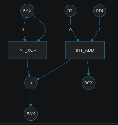
We can notice on this graph that:
- It is much simpler than the P-Code!
- The permutation of instructions has no impact on the graph.
The Phi-node, however, leaves us puzzled: nothing tells us what makes EAX set to zero or to the sum of RDI and RSI. That's expected, since the data flow is not sufficient to express the semantics of the code. We therefore add control flow edges to the graph:
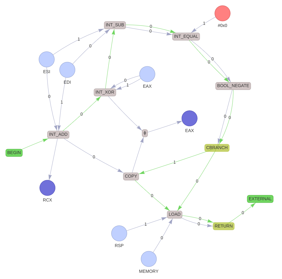
In the resulting graph, in addition to the condition for writing EAX, we also see the return address loading from the stack. The EXTERNAL node expresses the jump to an address outside of the code present in the graph. If the code does not end with a branch, we will have an END node. In total, we have ten different node kinds:
class NodeKinds(Enum):

    InputRegister = 0
    OutputRegister = 1
    Constant = 2

    Operation = 3
    Phi = 4

    ReadMemory = 5
    WrittenMemory = 6

    Begin = 7
    External = 8
    End = 9
There can be several memory nodes in a graph, but as no pointer aliasing analysis is performed we do not distinguish between memory addresses.
You may have noticed that adding the control flow edges breaks the invariance of the graph with respect to instruction permutations. We are thinking about improving the graph format to fix this. We are saving that for a future release of pcode_graph.
The CISCO TALOS dataset
This USENIX2022 paper introduces a dataset including a large corpus of binaries compiled across:
- 6 architectures (x86, ARM, MIPS)x(32 and 64 bits);
- 8 compiler variants (4 for gcc and 4 for clang);
- 5 optimization levels (O0, O1, O2, O3, Os).
The functions were extracted using IDA. In total, we have:
- 256,625 functions for training;
- 12,736 functions for validation;
- 522,003 functions for testing.
They also publish a comparison of 10 state-of-the-art approaches on this dataset.
Extracting the graphs
To speed up the training of our models, we start with a preprocessing step to extract the CDG graphs corresponding to the 791,364 functions of the dataset.
To extract the graphs, we use the LIEF library to extract the code at the offsets given by the dataset, then the make_graph_from_binary function to lift the code into P-Code and create the graph:
from pcode_graph.lief_importer import lookup_chunk
from pcode_graph.maker import make_graph_from_binary
from pcode_graph.translator import Translator

for arch, binaries in dataset_index.items():
    translator = Translator(arch)

    for binary_path, functions in binaries.items():

        binary = parse_binary(binary_path)

        for name, start, end in functions:
            code = lookup_chunk(binary, start, end)

            cdg = make_graph_from_binary(translator, code, start)

            output_path = compute_graph_path(dataset_dir, binary_path, name)
            output_path.write_bytes(pickle.dumps(cdg))
Lifting binaries into P-Code with pypcode is trivial in a simple case, but properly handling the presence of data in the middle of the code, or errors in function extraction heuristics, is not so simple. You can have a look at the code of the Translator class if you are interested.
The make_graph_from_binary method accepts options to guide the graph construction. In particular you can control the names of the registers whose writes should be considered as outputs of the code. If what you are extracting is a gadget, all registers can be useful, including processor flags. For our experiment, we used the default behavior which considers all the general purpose registers, but since we are interested in the semantics of a function, it would have been smarter to keep only the registers holding the return value, in order to simplify the dataflow graph while reducing the risk of bias.
This step takes time but parallelizes nicely via a small helper:
def run_in_parallel[P, R](
    function: Callable[[P], R],
    parameters: list[P],
    num_jobs: int | None = None,
    initializer: Callable = lambda: None,
) -> Iterator[R]:
    with multiprocessing.Pool(processes=num_jobs, initializer=initializer) as pool:
        for result in pool.imap_unordered(function, parameters):
            yield result
To avoid spending too much time on some very large functions of the dataset, we set a 5-second timeout for the analysis, the graph construction and its simplification. This removes 1.4% of the functions from the dataset.
Note that trying to lift a binary into P-Code while specifying the wrong architecture can give surprising results, so we had to detect and skip the 316 labeling errors of the training set.
Message-passing and diameter
A graph neural network (GNN) learns a representation of each node through the so-called message passing technique, that is, by iteratively aggregating the information of its neighbors. Starting from an initial state, each node aggregates the states of its direct neighbors to update its own state.
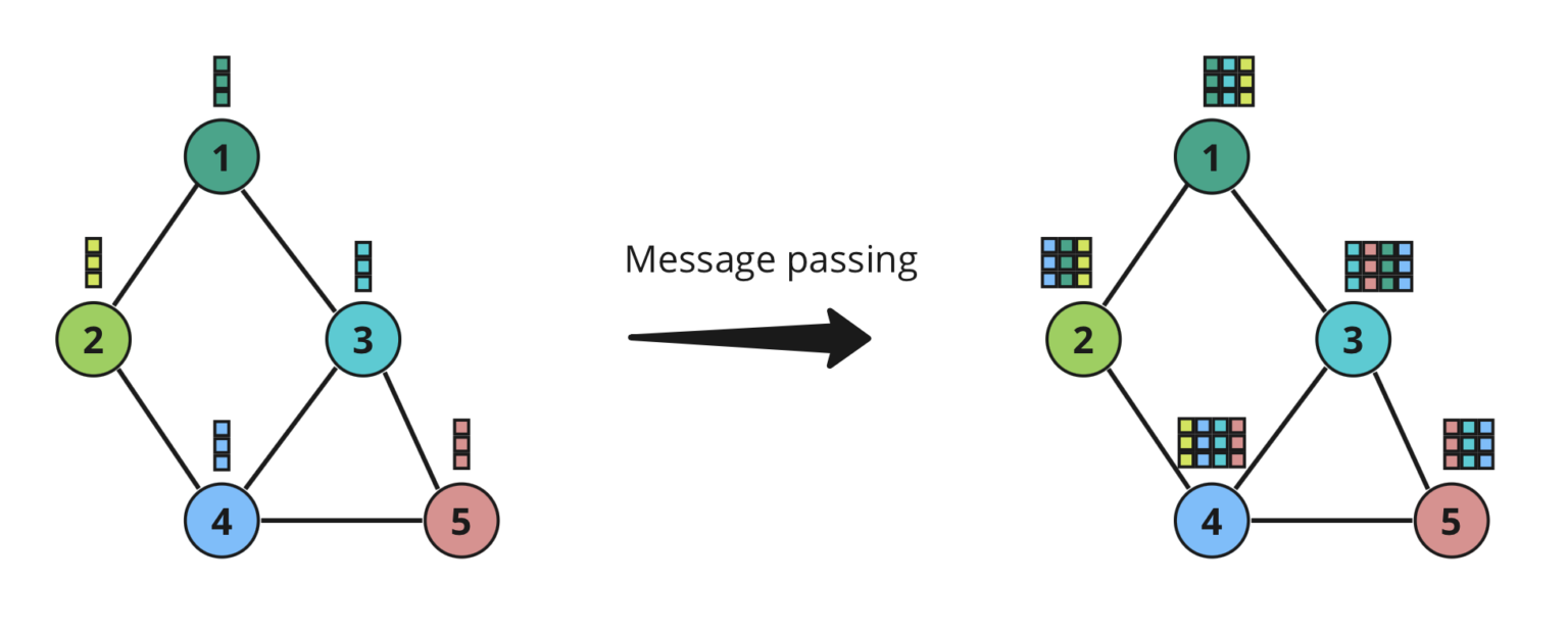
This aggregation is done via a graph convolution operator. We use the torch_geometric library, which provides an implementation of a good part of the research on the topic:
By stacking K convolution layers, a node ends up integrating the information coming from its K-hop neighborhood, while taking the topological structure of the graph into account.
Then, we can combine the resulting stats of all nodes to generate a global graph representation. This last stage is called readout.
To extract non-local properties of large graphs, one therefore has to stack many layers. However, unlike classical neural networks, GNNs suffer from an oversmoothing problem when the number of hops increases (> 10 layers). This is one reason why we strive to produce graphs with the smallest possible diameter, independently of their size.
To get an idea, here is the distribution of graph diameters on the validation set when considering only the control-flow edges, only the data-flow edges, or both:
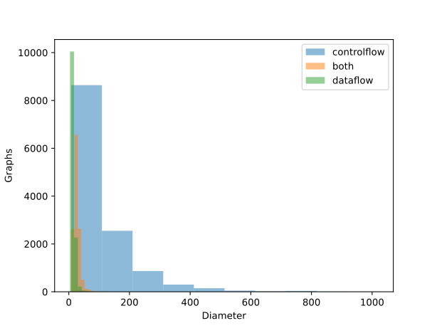
We notice that adding the control-flow to the graph slightly increases the diameter, but dataflow edges help limit the damage.
GNN architecture
GNN architecture remains a vast research topic and searching for the best hyper-parameters takes time. We simply used GINE to have a solid baseline:
from torch import Tensor, relu
import torch
from torch_geometric.data import Data
from torch.nn import (
    Dropout,
    ReLU,
    Linear,
    Module,
    ModuleList,
    Sequential,
)
from torch_geometric.nn import GINEConv, global_add_pool, GraphNorm
from dataclasses import dataclass


@dataclass
class GNNConfig:
    readout_head_outputs: int = 256
    head_hidden: int = 256
    conv_hidden: int = 64
    conv_layers: int = 4
    feature_dropout: float = 0.5


class GINE(Module):
    def __init__(self, config: GNNConfig, node_features: int, edge_features: int):
        super().__init__()
        self.convs = ModuleList()
        self.norms = ModuleList()
        self.dropout = Dropout(config.feature_dropout)

        for i in range(config.conv_layers):
            dim_in = node_features if i == 0 else config.conv_hidden
            self.convs.append(
                GINEConv(
                    Sequential(
                        Linear(dim_in, config.conv_hidden),
                        ReLU(),
                        Linear(config.conv_hidden, config.conv_hidden),
                    ),
                    train_eps=True,
                    edge_dim=edge_features,
                )
            )
            self.norms.append(GraphNorm(config.conv_hidden))

        self.head = Sequential(
            Linear(config.conv_hidden * config.conv_layers, config.head_hidden),
            ReLU(),
            Dropout(config.feature_dropout),
            Linear(config.head_hidden, config.readout_head_outputs),
        )

    def forward(self, data: Data) -> Tensor:
        hs = []
        x = data.x
        for conv, norm in zip(self.convs, self.norms):
            x = conv(x, data.edge_index, data.edge_attr)
            x = relu(norm(x, data.batch))
            x = self.dropout(x)
            hs.append(global_add_pool(x, data.batch))

        return self.head(torch.cat(hs, dim=-1))
Loss function
Now we have a model that computes an embedding of a graph, that is a fixed-size array of numbers associated with each graph of the batch passed to its forward method.
But it is not exactly what we need: to find similar functions we have to output a similarity score for a pair of functions.
We can do this by measuring the distance between embeddings, provided that the model was trained to push apart the embeddings of different functions while pulling together those of functions coming from the same program. Provided that our embeddings are L2-normalized, a dot is enough:
similarity = (emb1 * emb2).sum().item()
The classical method to produce this kind of embeddings consists in using a Siamese model and a Triplet Margin Loss. We went for a technique presented at NeurIPS2020: the Supervised Contrastive loss (SupCon loss).
Here is the loss and the final model, which wraps the former one:
from torch import Tensor, matmul, eq, eye, exp, log, clamp
from torch.nn import Module
from torch_geometric.data import Data
from torch.optim import AdamW
from torch.nn.functional import normalize


def supcon_loss(features: Tensor, labels: Tensor, temperature: float):
    """
    Supervised Contrastive Loss (Khosla et al., 2020).
    """

    # Similarity matrix
    # Should be already normalized
    # features = normalize(features, dim=1)
    logits = matmul(features, features.T) / temperature

    # Hack for numeric stability
    logits_max, _ = logits.max(dim=1, keepdim=True)
    logits = logits - logits_max.detach()

    # Compute mask of positive pairs (ie with same label)
    labels = labels.view(-1, 1)
    batch_size = features.shape[0]
    positive_mask = eq(labels, labels.T).float()
    self_mask = eye(batch_size, device=features.device)
    positive_mask = positive_mask - self_mask

    # Compute logprobs
    logits_mask = 1.0 - self_mask
    exp_logits = exp(logits) * logits_mask
    log_prob = logits - log(exp_logits.sum(dim=1, keepdim=True) + 1e-12)

    # Mean log_prob on positives for each anchor
    num_positives = positive_mask.sum(dim=1)
    mean_log_prob_pos = (positive_mask * log_prob).sum(dim=1) / clamp(
        num_positives, min=1.0
    )
    loss = -mean_log_prob_pos.mean()
    return loss


class SimilarityModel(Module):

    def __init__(self, num_node_features: int, num_edge_features: int):
        super().__init__()

        self.gnn = GNN(num_node_features, num_edge_features)
        self.optimizer = AdamW(self.gnn.parameters())

    def forward(self, graph_batch: Data) -> Tensor:
        """Returns normalized embeddings of binaries with given graphs."""

        z = self.gnn(graph_batch)
        return normalize(z, dim=1)

    def step(self, batch):
        emb = self(batch.graph)
        loss = supcon_loss(emb, batch.func_id, 0.07)
        self.optimizer.zero_grad()
        loss.backward()
        self.optimizer.step()
Translating the graph into tensors
The model consumes graphs in the torch.data.Dataset format. We still have to convert our CDG graphs to this representation. For that we use the graph_to_data function provided by pcode_graph.
This method has many parameters to adapt the node features to the task at hand. The most important one controls the way registers are encoded. Since our task only concerns the semantics of the functions, there is no point in including the registers other than those used by the calling convention: whatever the registers assigned to variables, what matters is what is the semantics of the code.
The map_calling_convention_registers function of pcode_graph makes it possible to encode the registers of the various calling conventions in a way that is consistent across architectures, so as to allow the model to generalize. It outputs an array of bits where each position corresponds to a use of the register: integer argument of rank n, 32-bit return value, etc. Note that a same register can be used both to pass a parameter and to return a value.
If your task only concerns a single architecture, you can simply use the map_registers function to convert a set of registers into hot-encoding. The idea is to send each possible value into a different input neuron, because it is much easier to teach a neural network a relation between its inputs than between different values of the same input.
Here is the code, sparing you the loading part of the dataset:
import pickle
from pathlib import Path
from typing import NamedTuple
from torch import Tensor
from torch.utils.data import Dataset
from torch_geometric.data import Data
from pcode_graph.gnn_exporter import graph_to_data, map_calling_convention_registers


class Function(NamedTuple):
    bin_path: str
    func_name: str
    func_id: int
    graph: Data


class FunctionDataset(Dataset):

    def __init__(self, csv_path: Path):

        super().__init__()

        # Load dataset from CSV
        self.graphs = []
        architectures = set()
        ...

        # Create register mappings of same size to have the same amount of node features for each arch
        self.register_mappers: dict[str, dict[str, Tensor]] = {}
        for arch in architectures:
            self.register_mappers[arch] = map_calling_convention_registers(arch)

    def __len__(self) -> int:
        return len(self.graphs)

    def __getitem__(self, index) -> Function:
        bin_path, arch, func_name, func_id, graph_path = self.graphs[index]
        graph = pickle.loads(graph_path.read_bytes())
        data = graph_to_data(graph, registers_emb=self.register_mappers[arch])
        return Function(bin_path, func_name, func_id, data)

    def __iter__(self):
        for i in range(len(self)):
            yield self[i]
Building the batches
The SupCon loss needs several examples per class in order to be able to compare positive and negative pairs within a same batch. We write a sampler to build balanced batches containing several samples of several different functions:
from collections.abc import Iterator
from itertools import islice
from random import Random
from torch.utils.data import Sampler

SEED = 42
SAMPLES_PER_FUNCTION = 4
FUNCTIONS_PER_BATCH = 16


class BatchSampler(Sampler):
    """Dataset PK sampling to produce batch suitable for use with SupCon loss."""

    def __init__(self, dataset) -> None:
        super().__init__()
        self.dataset = dataset
        self.rng = Random(SEED)
        self.num_batches = sum(1 for _ in self)

    def __len__(self) -> int:
        return self.num_batches

    def __iter__(self) -> Iterator[list[int]]:

        # Collect shuffles samples
        function_names = list(self.dataset.by_func_name.keys())
        self.rng.shuffle(function_names)
        samples: dict[str, list[int]] = {}

        for func_name in function_names:
            indices = list(self.dataset.by_func_name[func_name])
            if len(indices) >= SAMPLES_PER_FUNCTION:
                self.rng.shuffle(indices)
                samples[func_name] = indices

        # Build batches
        while len(samples) >= FUNCTIONS_PER_BATCH:
            batch = []
            to_delete = []
            for func_name, indexes in islice(samples.items(), FUNCTIONS_PER_BATCH):
                batch += indexes[-SAMPLES_PER_FUNCTION:]
                if len(indexes) >= 2 * SAMPLES_PER_FUNCTION:
                    del indexes[-SAMPLES_PER_FUNCTION:]
                else:
                    to_delete.append(func_name)
            for k in to_delete:
                del samples[k]

            yield batch
Training loop
In general, the crux for a fast training is to be GPU-bound, meaning that the performance of your tool is tightly correlated to the performance of your GPU. This can be achieved provided that computations and transfers are overlapped. There are plenty of libraries doing that, but a small torch function with a ping-pong buffer does the trick:
from torch.utils.data import DataLoader
from typing import Callable, NamedTuple
from torch import Tensor
from torch_geometric.data import Data


class BatchedFunctions(NamedTuple):
    bin_path: list[str]
    func_name: list[str]
    func_id: Tensor
    graph: Data


def apply_to_batches(
    dataloader: DataLoader,
    func: Callable[[BatchedFunctions], None],
    device: str,
):
    """Parallelizes computation and transfers with a ping-pong buffer,
    at the cost of a higher GPU memory consumption.
    """

    previous_batch: BatchedFunctions | None = None
    batch: BatchedFunctions

    for batch in dataloader:
        next_batch = batch._replace(
            graph=batch.graph.to(device, non_blocking=True),
            func_id=batch.func_id.to(device, non_blocking=True),
        )
        if previous_batch is not None:
            func(previous_batch)
        previous_batch = next_batch

    assert previous_batch, "No batch returned by dataloader"
    func(previous_batch)
And to put all the pieces together, the training loop:
from torch_geometric.loader import DataLoader

def train(device, csv_path):

    train_dataset = FunctionDataset(csv_path)
    train_data = DataLoader(
        dataset=train_dataset,
        pin_memory=device == "cuda",
        batch_sampler=BatchSampler(train_dataset),
        num_workers=16,
        persistent_workers=True,
    )

    model = SimilarityModel(train_dataset.node_features, train_dataset.edge_features)

    model.to(device)
    model.train()

    for e in range(config.num_epochs):
        apply_to_batches(train_data, model.step, device)
Note that the conversion from Function to BatchedFunctions is handled internally by the DataLoader.
Also note that to have a fully useful training pipeline you still have to incorporate:
- Evaluation on the validation set (after each epoch for instance);
- Logging (on tensorboard);
- Best model saving.
Evaluation method and results
The authors provide a list of negative or positive pairs for the validation and test subsets. The algorithms to benchmark have to return a similarity score for each of these pairs.
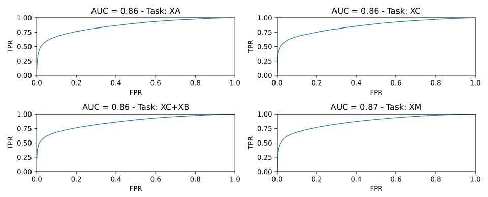
By varying the threshold beyond which the tested functions are predicted as coming from the same program, one can plot a ROC curve. The metric used is the area under this curve.
We obtain the curves below. To compare algorithms, the benchmark provides several tasks, The hardest one, XM, consists in mixing all the possible variations:
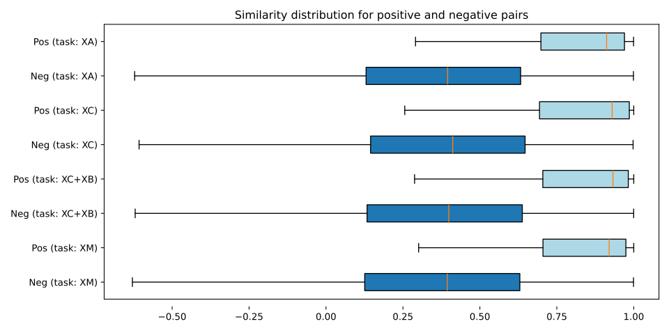
The drawing of the distributions of similarity scores obtained on each kind of pairs shows that positive and negative pairs are clearly separated:
And finally, we can compare our AUC score with the best one from the benchmark:
| Model | XC (same arch and bitness) | XC+XB (same arch) | XA (same compiler) | XM (different arch, bitness, compiler & optim level) |
|---|---|---|---|---|
| GMN | 0.86 | 0.87 | 0.86 | 0.87 |
| GINE 4 layers + pcode_graph features | 0.86 | 0.86 | 0.86 | 0.87 |
Doing the comparison is not completely honest because 1.5% of the bigger functions where just ignored in our case, but it seems that we achieve similar results that the best algorithm compared in the benchmark: GMN, for Graph Matching Networks.
This is not outstanding, but one could hardly expect more without working on the GNN architecture (and optimizing hyper-parameters at least a minimum).
Conclusion
This article shows how to use the pcode_graph library to generate binary code embeddings based on semantics. Even using an old GNN baseline, we got promising results.
We could go further by exploring more recent GNN architectures (like GATv2, DirGNN...) and doing a decent hyper-parameter search (number and size of layers, dropout probability, kind of normalization, readout operators, etc.).
Do not hesitate to fork the GitHub repository to adapt the library to your own use-case and feel free to send us feedbacks or submit issues.