Author Elie Mengin
Category Math
Tags binary analysis, machine learning, math, 2019
In this blogpost, we present a general method to efficiently compare functions from a new binary against a large database (made of numerous known functions). This method has strong theoretical properties and is perfectly suited to address many conventional problems, such as classification, clustering or near duplicate detection.
Introduction
Retrieving parts of a new binary executable that might be similar to some in other known programs is a major problem of binary analysis. Such feature has many application in different field of cybersecurity, such as vulnerability search, malware analysis, plagiarism detection, patch detection, etc.
For long, the problem has been entirely dealt manually by reverse engineers, but recent efforts and promising results suggest that part of the work - if not all - could be automatized.
If the very first techniques where based on the raw binary code, most recent approaches use graph-based representations of the program. Such representations have shown to be interesting trade-off between syntactic and semantic information describing the binary. In this blogpost, we focus on the analysis of each binary function independently. To do so, we use the conventional Control-Flow Graph (CFG) representation of the function, ie. an attributed graph which nodes are basic-blocks (consecutive sequences of instructions) and edges are jumps among them. Note that, in this work, we consider the functions as independent graphs, so we do not focus on the potential links between them (call procedures). This additional information would be used in further work.
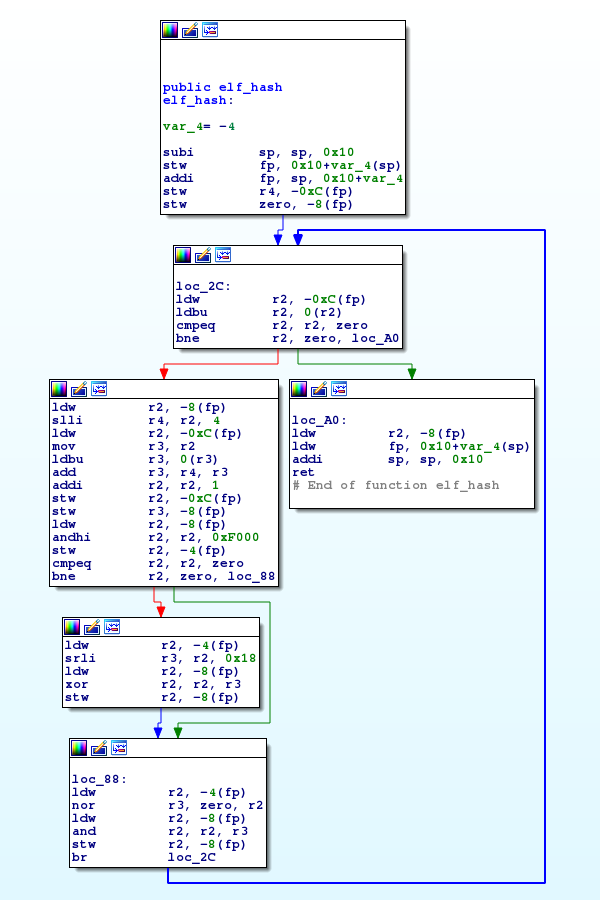
Figure 1: Once disassembled, each function can be represented as a graph made of basic blocks (nodes) and conditional jumps (edges).
In this blogpost, we present a general method to efficiently compare functions from a new binary against a large database (made of numerous known functions). This method has strong theoretical properties and is perfectly suited to address many conventional problems, such as classification, clustering or near duplicate detection.
Similarity measures in binary analysis
Mathematically, comparing functions requires that these later lie in a space that admits a proper measure of similarity. The definition of this measure is often considered one of the most important problem of binary analysis. Far from giving an exhaustive state of the art, we hereby briefly introduce some of the existing approaches to measure the similarity between functions. To do so, we distinguish the definition of similarity, which we present as an arbitrary characterization of the essence of the function, and the measure of similarity, a mathematical application that ultimately computes a similarity score between the two functions.
Regarding the definition of similarity, we distinguish two main considerations, namely the syntactic and the semantic characterization of the function. Note that most approaches use a mixed definition of the similarity, making these two groups non-exclusive:
On one hand, syntactic based definitions would consider similar two functions that share similar portions of code, similar basic-block layouts, etc. It often uses simple statistical features such as opcode counts or basic-block numbers, but can also involve more complex similarity descriptors, such as call birthmarks [1], MD-index [2], spectral embeddings [3], etc.
On the other hand, semantic based definitions focus on the intrinsic, essential meaning of the function, no matter the order of instructions or the basic-block structure. The main idea is to proceed to a reformulation of the sequence of machine-code instructions into a more unified ontology, that better describes its core functionality. Several reformulation approaches have been proposed, such as intermediate representation (IR) [4], tracelets [5], symbolic execution or taint analysis results [6], etc.
Once properly defined, the similarity has to be evaluated, ie. measured to produce a score. Again, we distinguish two different approaches.
The first one consists in depicting the functions as vectors in a normed space. Such vectors are often a simple concatenation of several arbitrarily designed features. Such features can describe the syntax (see examples above) just as well as the semantic of the binary (presence of specific instruction pattern, modification of the stack or registers, etc.), as soon as their comparison remains relevant. The similarity score is then computed using conventional vector-based metrics. One advantage of this type of approach is that, once the feature vectors are properly extracted, the similarity can be computed very efficiently. Moreover, when looking for similar items, many existing techniques allow to easily retrieve potential candidates, avoiding the computation of all pairwise similarity. On the other hand, any vector representation of a graph induces some information loss regarding its topology (the graph structure).
Another widely used approach consists in computing graph-based similarity scores. These scores often rely on the solution to an underlying graph problem such as graph edit distance, maximum common induced subgraph, longest common subsequence, linear or quadratic assignment, etc. Note that such scores might not be proper metrics. Although this approach seems more relevant, and the resulting similarity scores have shown to be of higher quality, this kind of methods is very costly to compute since it mostly relies on the resolution of hard combinatorial problems (most of them are at least NP-complete). It also requires more memory usage since each function is stored as a whole graph instead of a simple vector.
In the context of the comparison of a large amount of graphs, storing the graphs as well as computing all pairwise graph-based similarity scores quickly become prohibitive. However, we would appreciate a measure of similarity that favors topologically similar graphs. Thus, a suitable framework to measure function similarities would be a normed vector space in which each function is represented as a feature vector that efficiently encodes both its basic-block content and its graph structure. Moreover, this encoding and its corresponding measure of similarity should preferably respect the basic metric axioms.
In this blogpost, we introduce a method that respects these properties. This method is twofold. We first proceed a labelization of each nodes (basic-block) of the graphs using a locality-sensitive hash function. Then we vectorize the resulting labeled graph using a variant of the famous Weisfeiler-Lehman graph kernel. These two steps are separately presented in what follows.
Locality-Sensitive Hashing
As briefly mentioned here-above, our method aims at a vectorization of a graph via specific function, a kernel. The proposed kernel was originally designed for labeled graphs. A labeled graph is a graph which nodes are simple identifiers (strings or integers for instance), not necessarily unique. Since we choose to represent each function through its CFG, the graphs we would like to analyze are made of basic-blocks. Thus, we first need to give a label to each basic block before computing its kernel representation. Trivially, we could use a simple cryptographic hash function to give the same label to the same basic-blocks. Such a labelization scheme would not only lead to an exponential increase of different labels, but also distinguish very similar basic-blocks. For instance, consider two basic-blocks where the instructions have been equivalently reordered, or where a same instruction uses different registers. Using cryptographic hash function, those basic-blocks would be considered totally different whereas we might want them to be considered alike. In order to permit few changes in a basic block to be given the same label, we will use another labelization scheme, known as Locality-Sensitive Hashing (LSH) [7].
Basic-block representation
Let us first introduce our representation of a basic-block as well as our definition of similarity among them. Note that these definitions are purely arbitrary and that other considerations may be just as much legitimate as ours.
It is well known that the compilation of a same source-code may output different machine-codes that would though have the same overall behavior. Such resulting binaries are said to be semantically equivalent while syntactically different. These variations may be due to different targeted OS or architectures, different compiler versions, different compiling optimizations, etc. Usually, we consider four main possible alteration factors: addresses attribution, register usage, instructions reordering and optimization scheme [8] (such as peephole optimization, constant folding, loop optimization, function inlining, etc.). Thus, any measure of similarity between two basic-blocks should be as much independent as possible from these alteration factors. In our opinion, a satisfying solution to limit the impact of the three first factors is to simply ignore them (drop any address information, consider registers indifferently, ignore the order of instructions). However, efficiently detect and interpret alterations due to the optimization schemes is a much harder problem. If some heuristics could be used to track down known patterns, designing an exhaustive and automated method was out of scope in our work. Thus, we will mostly focus on a syntactic-based measure of similarity rather than a semantic-based one. It is worth noticing that even if not properly corrected during the simplification process, some alterations due to optimization schemes can be overcame by design in other steps of the method (the choice of the similarity measure, of the relabelization scheme, etc.).
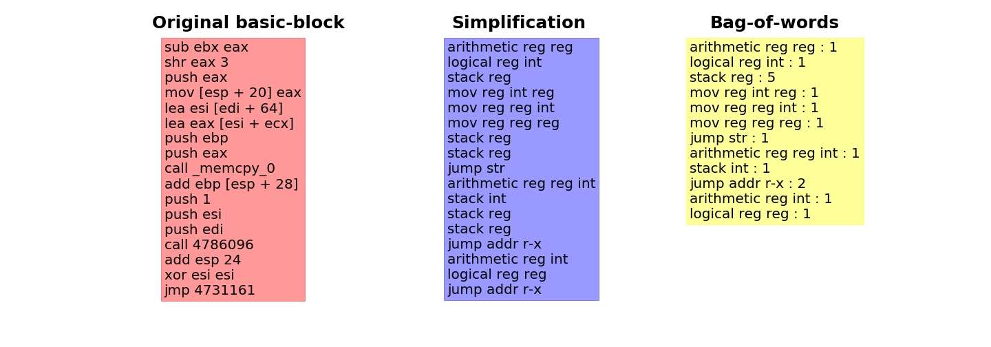
Figure 2: Left: In its original form, the basic-block contains many alteration factors that might heavily bias the retrieval of its nearest neighbors. Center: To limit the impact of these factors, we first proceed to a simplification by gathering the mnemonic by types as well as unifying any register names, address references or hard-coded string or numbers. Right: Once simplified, the basic-block is represented as a bag-of-words in order to ignore the instructions order. Note that the proposed simplification does not consider optimization schemes or known patterns. For instance, the penultimate instruction ``xor esi esi`` is semantically equivalent to ``mov esi 0`` and could have been reformulated as such.
Following these insights, we represent a basic-block as a set of instructions independently from its execution context or the object it may refer to (addresses, strings, etc.). Using such representation, each instruction (mnemonic + potential operands) can be seen as an element of a finite (though large) alphabet (or dictionary). Thus, each basic-block can be considered as a bag-of-words (the number of appearance of each word in a text) each of which have been drawn from this alphabet (see Figure 2). Note that the alphabet itself might be arbitrarily defined such that, for instance, look-alike instructions refer to the same words, or known sequence of instructions patterns are merged together into a single word. We now have a proper representation of a basic-block that limits the influence of most alteration factors and permits a large scale comparison with others. Note that this representation can be viewed as a large vector recording the number of all possible words in the alphabet. Let us now introduce our proposed labelization framework.
Random Projections
Recall that we seek at designing a labelization framework that gives the same label to similar inputs. A naive approach would consist in computing the distances from the input to all the known basic-blocks of the database and to determine a collision based on a threshold (if similar enough). Such approach would require at least operations and would thus quickly become prohibitive for a large enough. On the other hand, LSH techniques use probabilistic hash functions that collide similar inputs with high probability. Any label can thus be computed in operations.
Any LSH scheme is based on an arbitrary distance and can be seen as a dimension reduction that tends to preserve this distance. Similar inputs in the original space become equivalent items in the reduced one. Roughly speaking, it consists in a partition of the original vector space into "buckets", so that spatially close items (in the sense of the distance) are likely to end up in the same bucket, while dissimilar ones lie on different buckets. This framework trivially implies a surjection from the buckets to the labels. Unlike, conventional classification or clustering methods, this space partitioning is mostly computed irrespective of the input data and implicitly defines a great (or infinite) number of different buckets.
In practice, LSH techniques are widely used for nearest-neighbors search and near-duplicate detection problems. In this case, the hashing scheme is often completed by a query mechanism to limit the number of retrieved candidates (precision) while ensuring the presence of the nearest-neighbors among them (recall) [9]. Note that in our case, we only need to assign a label to each basic-block, so we will mostly focus on the hashing step and leave the query step untold.
In many LSH schemes, the space partitioning is computed using random projections. The idea is to randomly generate some hyperplanes and to encode each input with its position with regards to these hyperplanes. Close (similar) items have then higher probability to end up in the same bucket (space partition) since they are more likely to have the same relative position to the hyperplanes. The definition of the generative distribution of the hyperplanes as well as the encoding scheme depend on the distance one is willing to approximate. The number of hyperplanes (as well as the query mechanism) depends on the desired sensibility of the hashing process (maximizing precision or recall).
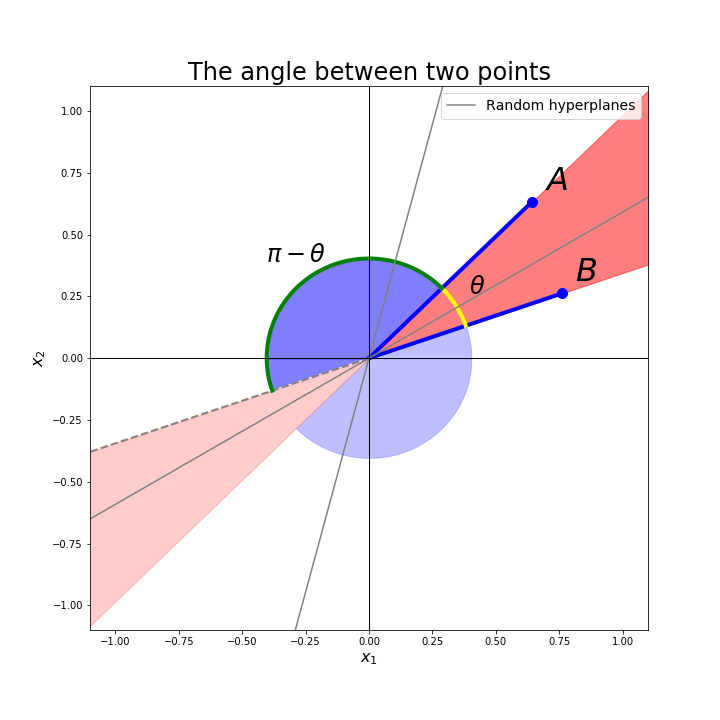
Figure 3: The probability that a random hyperplane (line in 2-dimensionnal space) lies between two points is proportional to the angle they form with the origin.
Two particular metrics are usually used for document near duplicate detection, the cosine similarity and the Jaccard index. In our work, we choose to use the cosine similarity to evaluate the distances between two basic-blocks. To approximate this similarity with LSH, we use uniform random projection. The idea is to compute the angle two points are forming with the origin. It is easy to show that this angle is equal to half the probability that a randomly generated hyperplane lies between the two points (see Figure 3).
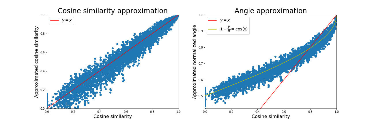
Figure 4: Left: The estimated cosine similarity using 256 random projections. Right: The relation between the estimated angle and the cosine similarity. For similar enough inputs, the angle accurately characterizes the cosine similarity. This later can thus be directly approximated using the estimated angle or corrected using a cosine function.
To efficiently encode the relative position of a point with respect to an hyperplane, one can simply keep the sign of its projection to this hyperplane. Hence, if two points share this same sign, it means that they both lie on the same side of the hyperplane, ie. it does not pass through them. Hence, by comparing the signs of the projections of two points to multiple hyperplanes, one can efficiently approximate the angle they are forming with the origin (see Figure 4). Depending on the desired result, one can approximate the angle using fast bit-wise (Hamming) comparisons or find the nearest neighbors using a bucket-based query mechanism.
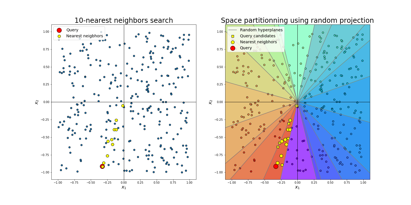
Figure 5: Left: Finding the k-most similar vectors to a query requires the computation of all pairwise cosine similarity scores. Right: With a partition of the space using uniformly generated hyperplanes, one can immediately retrieve some of the most relevant candidates. This partition can be use directly to hash the inputs or as a first filter to retrieve similar items.
In our case, we only seek at giving a label to each basic-block such that similar enough items have high probability to collide (see Figure 5). To define the desired ratio similarity/probability of collision, we usually use AND/OR amplification schemes. AND amplification schemes consist in the concatenation of several sign codes into a single label such that the probability of collision decrease exponentially with the similarity. On the other hand, OR schemes aims at allowing some sign differences, mostly by assigning several buckets to a same point. In practice, AND schemes usually improve the precision score but decrease the recall while OR schemes mostly do the opposite. Usually, both hash structures are used simultaneously. The resulting amplification can be easily computed (see Figure 6).
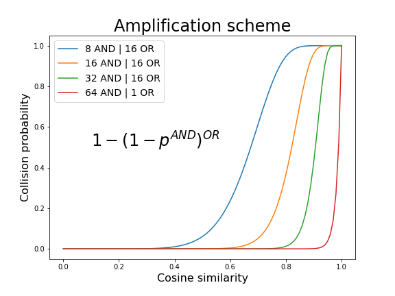
Figure 6: The probability of collision of two inputs according to their similarity. The desired accuracy can be set using AND/OR amplification schemes.
As an illustration, in a primary experimental work (10000 basic-blocks randomly taken from a large binary), we decided to target a 10%-sensitive hash function (we would like the function to give the same label to every basic blocks with cosine similarity above 0.9). Thus, we chose to use 32 randomly generated hyperplanes as well as an AND structure such that each label can be encoded in a 32 bits (unsigned) integer. Though very simple, this scheme achieved good results. We obtained a 98.4% precision score (the ratio of equally labelized basic blocks that are similar enough) with a 82.9% recall score (the ratio of similar enough basic blocks that are actually given the same label). Note that more complex schemes lead to better results but they require some query mechanisms that are out of scope in this blogpost.
Note that these results are given as an illustration of the precision/recall trade-off and do not augur of the overall performance of the proposed labelization technique in much larger and more heterogeneous configurations (different binaries, ages, developer's practices, compilers, optimizations, etc.). Note also that, while we wait for an in-depth analysis, it remains unclear to us if one should favors precision or recall (a tighter of larger partition of the space) to get the better results using the Weisfeiler-Lehman graph kernel [10] that we now introduce.
Weisfeiler-Lehman graph kernel
In the previous section, we introduced a method to efficiently labelize or retrieve similar basic-blocks. This local near-duplicate detection approach can be used to design a global graph analysis method that aims at encoding each function's CFG into feature vectors that are suited to large scale comparisons.
The representation of attributed graphs into a feature vectors is a whole field of study and several approaches have been proposed. In our case, we also require that this representation fits in a proper normed vector space in which the similarity among functions can be mathematically computed. Our feature map is inspired from an old method to compare graph with each other, namely the Weisfeiler-Lehman (WL) test of isomorphism.
Weisfeiler-Lehman test of isomorphism
For long, this test has been one of the most common techniques to check if two labeled graphs were isomorphic (have the same nodes and edges). The key idea is to iteratively compare the labels of each nodes' increasing-depth-neighbors. While these labels are equivalent, the two graphs are not proven non-isomorphic, and the algorithm iterates. For instance, the algorithm first compares the set of node labels of each graph (see Figure 7). If they are equal, it iterates. At the second iteration, it sorts then concatenates the labels of the neighbors of each node and compares the resulting set to the one of the other graph. Note that the labels are first sorted in order to avoid the intrinsic combinatorial property of graphs. The algorithm continues to iterate until the sets of labels are different (the graphs are then non-isomorphic), or it reaches the arbitrary maximum number of iterations. After a high enough number of iterations, the two graphs can be considered isomorphic (although in some rare cases, they might not be). Note that at each iteration, the resulting labels are compared regardless of any order. Hence, the comparison is usually based on the sorted set of labels or the number of appearances of each unique label (counter).
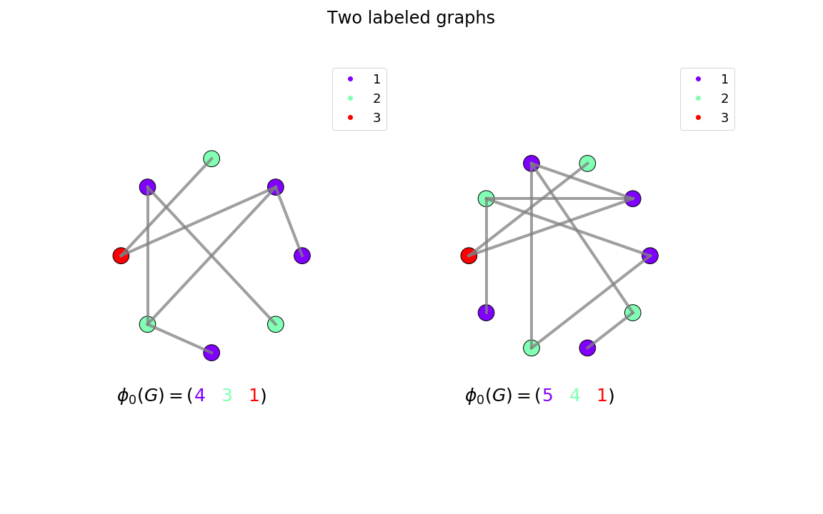
Figure 7: Two labeled graphs one would like to evaluate the similarity. Note that the two graphs are obviously not-isomorphic since they do not have the same number of nodes. Note also that for the sake of simplicity, we introduce undirected graphs but the method trivially generalizes to directed graphs.
An immediate limitation of this test is that the cost of computing the -depth-neighbors rises exponentially with . To overcome this issue, a trick consists in relabeling each node at iteration t with the compressed labels of its neighbors at iteration t-1 (see Figures 8-9). Using this scheme, each iteration runs in O(m), where m is the number of edges of the graph. Furthermore, this relatively simple, linear time algorithm is known to accurately detect isomorphism on almost every graphs.
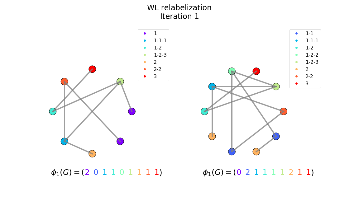
Figure 8: The relabeled graphs after the first iteration of the WL test of isomorphism. Each new label is made of the sorted concatenation of its neighbors labels at the previous iteration.
A major advantage of the Weisfeiler-Lehman test of isomorphism is that it can trivially be modified to allow one-vs-many test of isomorphism. Indeed, the iterative results of the relabelization/propagation procedure can be summed up in a large vector that thus fully characterizes the graph. Two identical vectors would thus indicate two isomorphic graphs (at least up to iterations of the WL test).
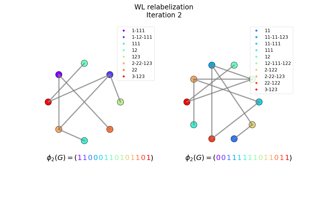
Figure 9: The relabeled graphs after the second iteration of the WL test of isomorphism. We may assume that comparing the resulting labels can provide information on the similarity of the two graphs.
Weisfeiler-Lehman graph kernel
Although initially designed to detect pure isomorphisms, this accurate, linear time procedure to characterize the topological information of a labeled graph has inspired further researches on graph similarity measure and graph comparison in general. Intuitively, a reasonable assumption is that two similar graphs would have a more similar WL vector representation than two different ones. We know describe our vectorization framework, as well as some of its properties.
Let us first recall our context of analysis. Suppose we are given a binary. This later is first disassembled and partitioned into functions. Each function is then represented using its control-flow, ie. as a graph, made of nodes (basic-blocks) and edges (jumps). Each basic-block is finally converted in a simpler semantic and represented in a bag-of-words form. As mentioned earlier, the WL test of isomorphism is designed to work on labeled graphs. Thus, we have to give a label to each basic-blocks. We choose to use a LSH labelization scheme similar to the one we introduced in the previous section.
Just as in the WL test procedure, the first iteration consists in concatenating the resulting labels. The algorithm then iterates. In the second iteration, we must give a label to the set of immediate neighbors of each basic-blocks. To do so, we choose to introduce a slight variant of the original WL procedure. Instead of grouping and sorting each basic-block's neighbors labels to create a new label, we choose to add the neighbors bag-of-words to create a virtual larger basic-block and to labelize this later using our LSH hash function. The resulting labels are then stacked to the ones of the previous iteration. The algorithm can go on. At the end of the -th iteration, each function is characterized by a vector of labels. This vector characterizes the whole graph, by encoding both content-based and topological-based information. We now want to compare it with each others.
Now that we transformed each function graph into a vector, we must define a proper measure of similarity that computes the similarity scores among these vectors. This appears not to be trivial. Indeed, the vectors might be of different sizes (depending on the number of basic-blocks composing the function), the similarity and no obvious measure of similarity can be defined between different labels. In such cases, it is common to define a label-wise metric ie. a metric that measures the similarity of each label's number of appearances among the two vectors. Local similarity scores are first computed independently (label by label), and then added altogether to give an overall similarity score. This later summation can be viewed as an inner product norm over a virtual vector of label-wise similarity. Following this definition, each vector can be viewed as feature map, ie. a high (potentially infinite) dimensional function that takes a graph as input and outputs the number of appearances of each label according to the WL procedure.
Since the vectors are compared label by label using an inner product norm, their dimension should be the number of all possible labels. This number is very large, and potentially infinite (depending on the labelization scheme we use), since one can always design a basic-block so different from all others that it would be given a new label. Although infinite dimensional, feature maps are perfectly suited for the computation of inner products since it only has to sum the product of non-zero values (few coordinates over an infinite-dimensional vector). Thus, a suitable vector space to properly compute the similarity of WL vectors would be a high-dimensional, complete and normed vector space with a proper inner product. Such a space is also known as an Hilbert space.
The relative simplicity of the inner product might prevent from accurately computing the underlying similarity among two vectors. In this case, we may want to use a finer norm while preserving the properties of an Hilbert space. For instance, we might consider the presence of some labels as more relevant than others and proportionally increase their contribution to the similarity score. We might also want to use more complex non-linear norms. To do so, it is common to introduce a new higher-dimensional Hilbert space which feature maps inner product is equivalent to the non-linear norm in our original space. Note that this new space may remain abstract since we ultimately want the value of the inner product in it (the value of the desired norm in the original space). Not every norms can be represented as an inner product in a higher dimensional space. In fact, by the Moore–Aronszajn, this norm must be positive semi-definite [11]. Such a norm is then called a kernel and the induced Hilbert space is called a Reproducing Kernel Hilbert Space (RKHS) [12]. Note that our original space is also an RKHS since the linear kernel (the inner product) is positive semi-definite.
Besides allowing large scale comparison using fast inner product measures and almost transparently enabling more complex non-linear norms, the introduction of RKHS provides some interesting properties when addressing several statistical optimization problems. We briefly introduce these properties in what follows.
Properties of the RKHS
Recall that from now, we designed a vectorization technique that takes a graph as input, and outputs a feature maps, ie. a vector that records the number of appearances of each labels according to our WL procedure. Although the dimension of this vector is very high, computing its similarity with another vector is straightforward since we use an inner product norm. In order to use a more complex non-linear norm, we can also introduce an abstract higher-dimensional vector space which inner product norm is equivalent to the desired non-linear norm in the original space. However, this norm must be a positive semi-definite kernel. The new abstract space it induces is then called Reproducing Kernel Hilbert Space and possesses some interesting properties [13].
Indeed, it can be shown that, according to the kernel's reproducing property, any function of a vector in the RKHS can be written as a linear combination of the kernel evaluation over this vector and all others. In other words, any function of an infinite dimensional vector in the RKHS can be written as a weighted sum of inner products between this vector and the few others. An immediate corollary of this property is that any linear optimization problem in the RKHS can be easier to solve using its finite linear combination form than its primal infinite dimensional one. Moreover, the Representer Theorem states that, in the RKHS, as long as the objective function is penalized, it admits a unique minimizer. Note that these properties hold for any RKHS, ie. for any positive semi-definite kernels, even non-linear ones.
These properties make this framework very appealing to approach all kinds of linear optimization problems such as graph classification or graph clustering. It is also particularly suited to solve max-margin problems using Support Vector Machines. Note that the vectors can also be used in their primal form to compute similarity or find near neighbors.
Conclusion
In this blogpost, we proposed a new approach to address several binary function analysis problems. It is designed to work on functions represented using their control-flow graph. The main idea is to transform each attributed graph into a vector that efficiently encodes both its basic-block content as well as its topological structure. This conversion is done using a slight variant of the famous Weisfeiler-Lehman graph kernel. In their vector form, the functions can be compared efficiently, even in large databases. Since the WL kernel is Mercer, it has important properties that allow to efficiently address many conventional problem such as classification or clustering. It is also suited to perform function near duplicate retrieval, an important problem of binary analysis.
The proposed method is inspired by a kernel initially designed for labeled graphs. Thus, we introduced a probabilistic labelization scheme that aims at assigning the same label to similar basic-blocks. Designed to work on very large databases, this scheme performs in operations, hence prevents to compute the distance to all previously known basic-blocks. We also mentioned that these scheme is also perfectly suited to the more conventional basic-block near duplicate detection problem though we did not give further details.
Recall that this hashing scheme is designed to approximate a particular measure of similarity (cosine) and that this similarity is evaluated on an arbitrary choice of features that could be discussed. We also briefly gave some insights on the problem of defining and measuring the similarity between two binary functions or two basic-blocks.
We have not yet proceed a extended empirical evaluation of our approach. More results would certainly be given on further publications.
Thanks
A big thanks goes to my colleagues at Quarkslab for proof-reading this blog post.
References
| [1] | Choi, S., Park, H., Lim, H. I., & Han, T. (2007, December). A static birthmark of binary executables based on API call structure. In Annual Asian Computing Science Conference (pp. 2-16). Springer, Berlin, Heidelberg. |
| [2] | Dullien, T., Carrera, E., Eppler, S. M., & Porst, S. (2010). Automated attacker correlation for malicious code. BOCHUM UNIV (GERMANY FR). |
| [3] | Xu, X., Liu, C., Feng, Q., Yin, H., Song, L., & Song, D. (2017, October). Neural network-based graph embedding for cross-platform binary code similarity detection. In Proceedings of the 2017 ACM SIGSAC Conference on Computer and Communications Security (pp. 363-376). ACM. |
| [4] | Dillig, I., Dillig, T., & Aiken, A. (2009). SAIL: Static analysis intermediate language with a two-level representation. Technical Report, Tech. Rep. |
| [5] | Omer Katz, Ran El-Yaniv, and Eran Yahav. 2016. Estimating types in binaries using predictive modeling. SIGPLAN Not. 51, 1 (January 2016), 313-326. |
| [6] | Cova, M., Felmetsger, V., Banks, G., & Vigna, G. (2006, December). Static detection of vulnerabilities in x86 executables. In 2006 22nd Annual Computer Security Applications Conference (ACSAC'06) (pp. 269-278). IEEE. |
| [7] | https://en.wikipedia.org/wiki/Locality-sensitive_hashing |
| [8] | https://en.wikipedia.org/wiki/Optimizing_compiler |
| [9] | https://en.wikipedia.org/wiki/Precision_and_recall |
| [10] | Nino Shervashidze, Pascal Schweitzer, Erik Jan van Leeuwen, Kurt Mehlhorn, and Karsten M. Borgwardt. 2011. Weisfeiler-Lehman Graph Kernels. J. Mach. Learn. Res. 12 (November 2011), 2539-2561. |
| [11] | https://en.wikipedia.org/wiki/Positive-definite_kernel |
| [12] | https://en.wikipedia.org/wiki/Reproducing_kernel_Hilbert_space |
| [13] | https://en.wikipedia.org/wiki/Kernel_method |