Authors Tom Czayka, Romain Thomas
Category Android
Tags Android, binary diffing, tool, 2019
This blog post is about how to efficiently spot code mutations between distinct versions of an Android application.
We are starting a blog series that addresses similarity detection in Android applications.
This first blog post exposes concepts and designs behind the diff engine developed at Quarkslab. The second will show a concrete use case about identifying the patch for a recent vulnerability: CVE-2019-10875. Finally, the last one will explain how we took advantage of Redex, in association with our diff tool to detect modifications within an obfuscated application.
Introduction
Detecting similarities is not a brand-new problem and has been already covered by several academic papers as well as tools like BinDiff, Diaphora, YaDiff and so on. The presentation by Joxean Koret titled "Past and Present of Program Diffing" [1] gives a good overview of the state of the art.
Regarding Android applications, some tools and frameworks already exist but as far as we are aware, they are not as mature as diffing tools for native code.
Similarity detection can have different purposes like identifying one function inside a set or detecting a library or a third-party SDK within an APK. In our case, we are in the context in which we aim to spot mutations among two sets of classes or methods extracted from two distinct versions of an APK.
The results of the diff can be used to detect patching of vulnerabilities, to reverse engineer obfuscated code -like what is outputted by Proguard- based on prior analysis, or to identify repackaging of applications.
In the first section, we introduce the challenges of spotting similarities in APKs compared to native code. The second part provides a technical overview of our diff engine. Finally, the last part shows some performance results based on genuine applications.
Challenges when implementing a diff engine
Unlike assembly code, the Dalvik instruction set is quite verbose and the structure of the bytecode makes analysis easier than with native code. For instance, in the Dalvik bytecode it is straightforward to access method strings while in native code we have to deal with relocations, sections, etc.
However, Android applications are becoming bigger which leads to the adoption of multiple .dex files [2]. The first challenge we need to overcome is to efficiently handle the multi-DEX structure of applications. As the implementation can be split into different DEX files, we have to resolve and provide a unified overview of the different classes and methods. As a result, we implemented a merge strategy that makes an abstraction over the multiple DEX files as if they were one.
The second challenge is about implementing a scalable diff engine that supports a large number of objects to compare. On recent Android applications, it is fairly common to embed tens of thousands of classes. For instance, Twitter v7.90.0 (released on April, 8th) contains no less than 36352 classes and 230185 methods divided into 5 DEX files. If we opt for a naive approach in which we compare the classes one by one, we would need operations, that is about operations for Twitter.
While the multi-DEX issue is mostly related to software engineering, the second involves both theoretical concepts and efficient implementation.
Let's now get into the technical overview.
Technical overview
In this part, we discuss how an Android application-oriented diff engine can be designed and built by taking advantage of several special aspects brought by the DEX format and the Dalvik instruction set. As this project focuses only on Android, the approach is specific and considers the benefits and constraints exposed previously. Therefore at some point the result will differ from regular native code diffing strategies.
In a first place and in order to accurately understand the implementation of our diff engine, we need to expose its purpose. The diff engine takes two sets of classes (from two APKs) as input and produces a list of matches as output. Each match contains a pair of two classes and the metric of similarity between them. The similarity is normalised to a floating point number between 0 and 1. The more the similarity tends to 1, the more similar classes are. Whenever distance is strictly equal to 1, we assume that it is a perfect match. It means that the two matching classes look exactly alike. When it comes to diff calculation, it implies that the class from the original APK and the class from the modified APK are the same — that is, developers have not altered the class in any way whatsoever. It is a crucial information because if we can out how similar classes are then we are able to focus analysis on the detected mutations.
Let's now dive into the internals of the diff engine. Technically speaking, it includes three main stages that allow us to quickly and efficiently compare two sets of classes: the first stage divides classes into clusters, the second performs a rough comparison whereas the last performs accurate comparison.
Prior to running these stages, we have the option to reduce the input sets of classes passed to the diff engine to enhance performance. This step can be important because it significantly affects the diff engine quality. The diff engine will be both faster and more likely to find divergences among two small sets than two large ones. In other words, the fewer the better. We will see why later through this post. As an example, one may reduce the sets of classes as follows:
v1, v2 = load("v1.apk"), load("v2.apk")

classes_v1 = filter(v1.classes, CONDITION)
classes_v2 = filter(v2.classes, CONDITION)

diff_result = diff(classes_v1, classes_v2)
Prior stage: Filtering classes
As applications often embed a bunch of external modules and third-party SDKs, the number of classes can be pretty huge. For instance, Twitter app contains 36352 classes but only 10078 are located in the package name com.twitter.android. However, most of the time, while inspecting an Android application, reversers have to focus only on specific parts or packages. This implies that lots of classes are irrelevant for analysis. In such cases it is pointless to compare all the classes as a broad category. Output would be full of results that we do not care about. Moreover, depending on application size, comparing too many classes will be both more resource-intensive and time-consuming. Thanks to Dalvik's design and the modularity model it borrows from Java [3], these features are usually already split up into different packages and this information can be retrieved from DEX files.
From our point of view, taking advantage of packages is a great way to reduce the input sets because inner package structure is unlikely to radically change across versions. By only selecting classes that really matter and skipping others we are able to make the sets drastically smaller. 1 illustrates this step. In this example, we only deal with classes in packages com.android.app.signup and com.android.app.webapi. Note that all nested packages such as com.android.app.webapi.ping are not represented here but are selected in the input sets as well.
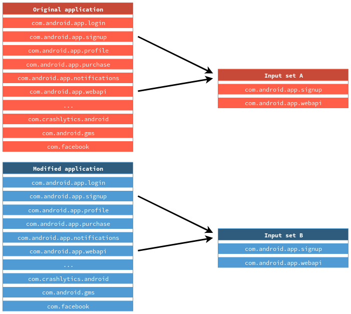 Figure 1. Filtering classes according to their package names.
Stage 1: Clustering
At this point, we have two sets of classes A and B selected for comparison. We can now get into the internals of the diff engine and expose the first stage that consists of dividing classes into several groups as much as possible. Those groups are called clusters and are built according to the package in which classes are located. If the classes PingRequest and PingResponse are both part of com.android.app.webapi.ping, they will be placed in the same cluster. Nonetheless, they won't be alongside neither SendPictureRequest nor AdsResponse which are respectively in com.android.app.webapi.picture and com.android.app.webapi.ads.
Then, each cluster from set A is linked to its corresponding one from set B according to their package name. A pair of two clusters makes what we call a pool.
Figure 2 outlines the results of this process.
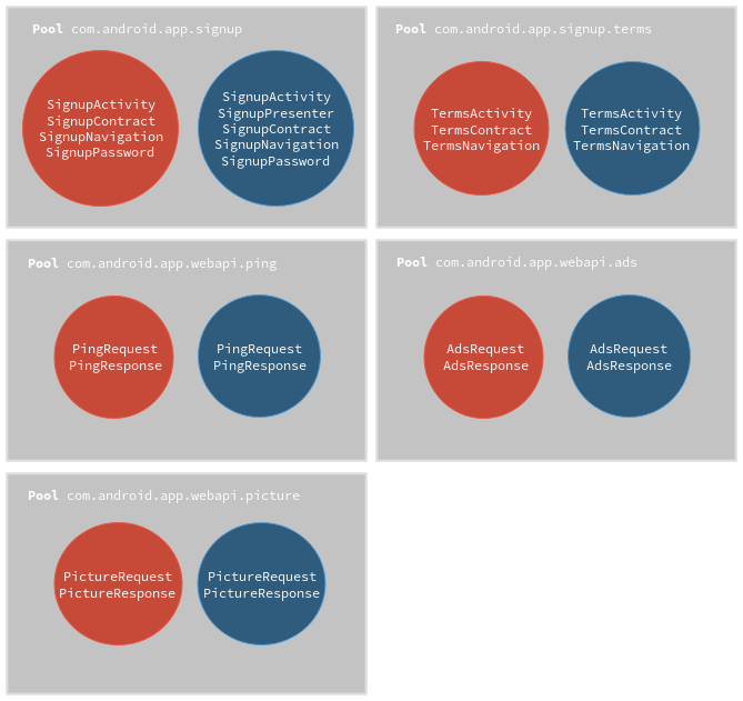 Figure 2. Results after clustering classes and creating pools.
That way, we are able to deal with pools of classes instead of flat sets of classes. Rather than comparing all the classes within the two input sets together, we work at pool scale which heavily reduces the overall number of comparisons and enables computation parallelism on pools.
However, this stage is not compulsory and could be skipped on specific situations. Indeed, if the application has been obfuscated by messing up package names and/or structures, pools become irrelevant. It is the reason why we tried to make our engine obfuscation-resilient as much as possible and hence develop a mechanism that aims to detect obfuscated names thanks to entropy calculation and package name length. As a result, classes from obfuscated packages are treated as a single cluster which affects overall performance as clusters get larger. Nonetheless, this scenario also has to be considered and resource and time consumptions must be reasonable.
Stage 2: Bulk comparison
After comparison sets have been optimized and reduced, we can start comparing classes within every pool. However, some pools may remain pretty large and may contain clusters of thousands of classes. Especially, when the application is obfuscated by flattening packages. Thoughtlessly comparing classes one by one would require lots of computational resources and time due to the complexity in . Thus, we need an efficient way to process them. To address this problem, we took inspiration from techniques applied for near-duplicate detection (e.g. Google web crawler for finding duplicate pages) and more exactly, we applied a SimHash-based algorithm [4]:
SimHash is a strategy for quickly estimating how similar two sets are. Given a set of input values, it produces a single similarity-preserving hash. This hash is quite interesting because two near input sets generate output hashes that are roughly identical. This similarity estimation can be calculated by computing the hamming distance between the two output hashes.
Regarding our case, this approach seems really valuable. Instead of comparing class features one at a time for every class, we would compute a single hash which represents a whole class, called class signature. Going further, it means that two classes could be compared by simply computing the hamming distance between their own signature. The closest the signatures are, the more similar classes are. Note that this operation is really cheap on modern CPU thanks to the x86 POPCNT instruction [5].
However, in order to produce such signature, a set of values has to be passed as input. Those values have to be wisely selected since they must accurately characterise the class. Fortunately, there is a large number of features that can describe a class: the number of fields, the number of methods, the method prototypes, the number of cross-references and so on. Note that those are only structure-related because embedded data such as class names, field/variable values (in particular strings) are heavily obfuscation-prone. It is better to not rely on these features in a first place.
Looking ahead to future improvements, we decided to generate four 32-bit partial hashes which form, once concatenated, a 128-bit class signature. Each partial hash represents a category of information. Indeed, we have there four categories of information:
Class: number of methods, number of fields, access flag, etc.
Fields: type, value set (if any), static visibility, etc.
Methods: number of arguments, number of cross-references, return type, etc.
Code: instruction opcodes.
Figure 3 shows the binary representation of a class signature and the four partial hashes it is composed of.
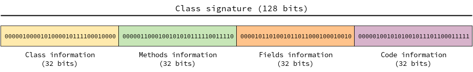 Figure 3. Binary representation of a class signature.
Thanks to that design we are able to compare classes at distinct levels. For instance, if we would like to compare two classes at field level exclusively, we just have to compute the hamming distance between the two partial hashes which correspond to fields information. Of course, we can also perform an overall comparison by considering the full class signature. Note that this model allows us to spread information over class signature as well.
Moreover, we treat each class individually. That is, we do not consider class relatives such as parent or child classes as the complexity would increase quite easily in such configuration.
Getting back to our initial concern: how can we find the class C' in a cluster which is the nearest-neighbour of class C in the other cluster? We are still facing performance issues as each class signature has to be compared with all others from the other cluster. Here comes the search strategy brought forward by Thomas Dullien from Google Project Zero [6].
He got roughly the same problematic but applied to native code. He also represents comparison items as signatures, and introduced the idea of estimating the nearest-neighbour by subsampling bits from signatures and creating hash families thanks to bitwise permutations (cheap operations). It allows us to build a list of hashes divided into several hash buckets. That way, we no longer have to compare elements one by one but instead, only with signatures that share common properties with the targeted one. Obviously, this technique is an estimation therefore there are odds of getting some wrong results depending on the number of buckets but it provides a great trade-off for bulk comparison. The more buckets we set, the more accurate the results are. Nonetheless, that still takes more resources and time.
Digging further into this algorithm, it is designed like a search feature. It needs to know initially which values could be looked for. Thus the first step is to register all signatures from a given cluster. To do so, we have to perform n permutations on each input signature where n is the number of buckets we want to use. We then keep in memory, in a sorted container, those different hashes and their permutation index which identifies the step during the permutation process. In order to identify the nearest-neighbours of a given signature S, we call the same permutation function and for each permutation, it iterates over the hashes located in the corresponding bucket described by the common first few bits. If a hash also shares the same permutation index, it is placed onto a list of candidates and the hamming distance between their initial signatures is computed and stored. As a result, we are finally able to get a list of nearest-neighbours of S, ordered by hamming distance.
Stage 3: Accurate comparison
At this point, we have got the n nearest-neighbours of our targeted class thanks to the latest stage. Nonetheless, as we previously explained, those results are just approximations based on class signatures. However, we aim to accurately know how similar the targeted class and its neighbours are. Not how close their respective signatures are. It would consequently consume resources and time but let's say that we choose to only keep three nearest-neighbours. A thorough comparison is totally practicable because for each class, it performs the comparison with three other classes at most. This approach significantly enhances the final result.
To do it we take the targeted classes' and neighbour's features described above one at a time and compute a similarity percentage between them. Then, an overall similarity average is computed thanks to those. At this stage, we can also consider additional features such as source file names or embedded strings depending on the situation and the kind of obfuscation.
We also have to take actual code into account — that is, compare class methods at Dalvik bytecode level. This part must be flexible enough to match codes across distinct compilations that could possibly use different instructions and different optimizations for the same input Java code. Hence, we implemented an abstraction layer as a categorisation mechanism for instructions. In other words, each instruction opcode is classified according to the kind of operation it executes. For instance, there are a bunch of invoke-* opcodes [7] which could cause divergences during comparisons whereas developers did not modified the related Java code. Thus, instead of dealing with the raw opcodes, we work with what we call abstract opcodes. They represent the following operations:
None (like nop)
Test (like if-eq, if-ne)
End of basic block (like return-object, throw)
Comparison (like cmp-long, cmpl-float)
Call (like invoke-virtual, invoke-static)
Arithmetic (like neg-int, not-int)
Cast (like int-to-float, int-to-double)
Static field access (like sget-object, sget-boolean)
Instance field access (like iput-wide, iput-byte)
Array access (like new-array, filled-new-array)
String (like const-string, const-string/jumbo)
Move (like move-wide/16, move-wide/from16)
Integer (like const/16, const/4)
Note that we do not consider registers because they are likely to change between different compilations. Now, we collect all abstract opcodes of all class methods as a sequence of bytes and concatenate the whole thing in order to represent the code embedded within the class. The purpose of this operation, is to compare these byte sequences with a known string distance algorithm. It turns out that problems may happen when the methods order differs across versions: a given method may appear first in version 1.0 but third in version 1.1 without any Java modification.
Therefore, we have to sort this out beforehand. To do so, we generate a 16-bit signature which stores the number of instructions the method has and the XOR operation result of every opcode it contains. Then, after numerically ordering those signatures, we are able to establish the final byte sequence for each class. These can be effectively compared thanks to Levenshtein algorithm [8] which outputs the distance between them. This distance is then added to the overall similarity average described above.
Lastly, the neighbour that produces the highest overall similarity average is defined as the actual match. The distance between these is the normalised percentage.
Assessment
In order to properly assess our complete tool, we have performed comparisons between minor versions of several well-known applications. It only compares computation time as result. Effectiveness will be evaluated through the next blog posts. The following table shows obtained results for three selected applications. Note that Loading time represents the time spent for loading both original APK and modified APK. The load() operation involves DEX parsing, bytecode disassembling and multi-DEX resolution.
| App name | Compared classes | Loading time (ms) | Diff time (ms) |
|---|---|---|---|
| Microsoft Authenticator | 1662 | 2250 | 337 |
| Lime Bike | 4503 | 2621 | 685 |
| 4919 | 5308 | 810 | |
| 12701 | 5295 | 3241 | |
| 27390 | 5304 | 152029 |
References
| [1] | https://docs.google.com/presentation/d/19h0T8BBn_96ZkdclFHV_MSgLPSGRrbWJpU_99heav88 |
| [2] | The DEX format uses 16-bit integer to store numbers of classes, methods and so on. Hence, it is bound to 65535 objects |
| [3] | https://docs.oracle.com/javase/tutorial/java/concepts/package.html |
| [4] | http://www.cs.princeton.edu/courses/archive/spring04/cos598B/bib/CharikarEstim.pdf |
| [5] | https://www.intel.com/content/dam/www/public/us/en/documents/manuals/64-ia-32-architectures-software-developer-instruction-set-reference-manual-325383.pdf#G7.572223 |
| [6] | https://googleprojectzero.blogspot.com/2018/12/searching-statically-linked-vulnerable.html |
| [7] | https://source.android.com/devices/tech/dalvik/dalvik-bytecode.html#instructions |
| [8] | http://people.cs.pitt.edu/~kirk/cs1501/Pruhs/Spring2006/assignments/editdistance/Levenshtein%20Distance.htm |