Authors Roxane Cohen, Robin David, Riccardo Mori
Category Program Analysis
Tags reverse-engineering, binary diffing, tool, 2023
This blog post presents an overview of QBinDiff, the Quarkslab binary diffing tool officially released today. It describes its core principles and shows how it works on binaries as well as on general graph matching problems unrelated to IT security.
QBinDiff: A modular diffing toolkit
Introduction
Binary diffing is a specific reverse-engineering task aiming at comparing two binary files that are usually executables. The ultimate refinement of disassembly, baring decompilation, is usually the recovery of functions with bounds along with the associated call graph. As functions represent the different functionalities contained in a binary, they are usually used as the base artifact for diffing. The goal of differs is to compute a mapping between functions of a first binary called primary (A) against those of the second called secondary (B). The mapping computed is usually a 1-to-1 assignment. More evolved approaches try to compute M-to-N assignments as functions can be inlined, or split by means of compilation or obfuscation. This blog post focuses on the 1-to-1 assignment case.
Diffing somehow requires comparing the two programs and their functions. So the main question is: which criteria should be used to match two functions? A differ like Diaphora is applying successive comparison passes starting from the most empirically accurate (function names, bytes hashes, etc...). BinDiff, instead, is heavily relying on the call graph and starts from imported functions as anchors. It then explores recursively their call graph neighbors to match functions.
While they work very well in most usual cases, they reach some limits on more specific scenarios (e.g.: two banks in the same firmware) or altered binaries like obfuscated ones. Consequently, in the past few years, we explored alternative diffing algorithms that would be more customizable in these scenarios where the reverser might be led to provide their own features and criteria to perform the diff.
This led to the development of QBinDiff, a customizable, yet experimental, differ.
Diffing as an instance of more generic problems
Formally, we define the graph-matching problem as the process of aligning two attributed directed graphs, where the term align means finding the best mapping between the nodes of the first graph (called primary) to the nodes of the second one (called secondary). In this case what exactly characterizes the best mapping is intentionally left undefined as there are multiple ways of defining what a good match (between two nodes) is. It usually depends on the nature of the underlying problem instance solved. For example, in binary diffing we might consider a match between two functions to be good (aka valuable) if the two functions are semantically equal or similar enough, although, on the other hand, we might also be interested in evaluating how much they syntactically differ, hence, a good alignment has to leverage the similarity between the nodes. In other scenarios, instead, we might be more focused on the topological similarity of the two nodes, which means relying less on the node attributes and more on the call graph (i.e.: graph topology).
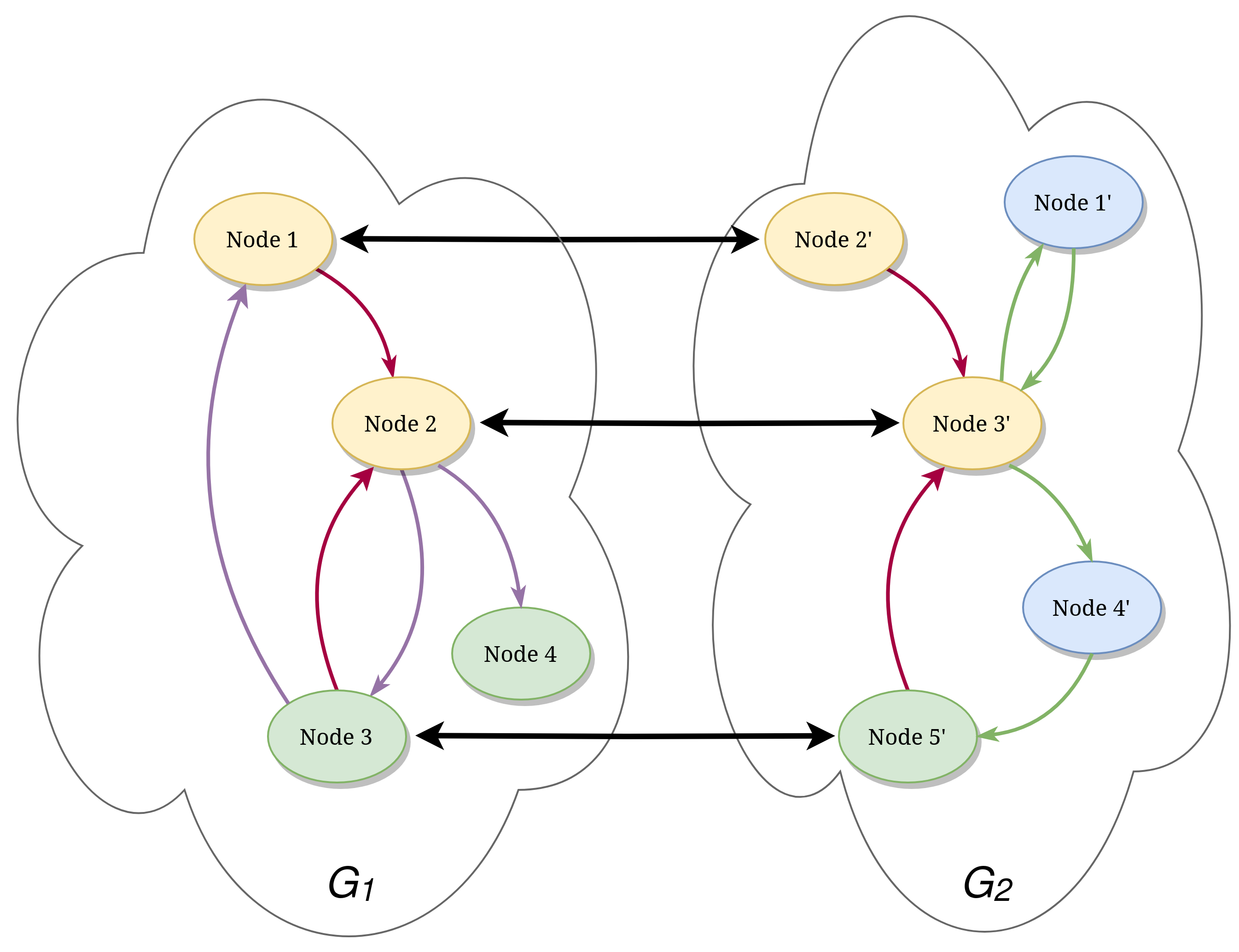
In the previous image, we can see a representation of the graph alignment problem where we are considering both topological information (the edges) and node attributes (the colors). The black bold arrows represent the alignment (mapping).
The graph alignment problem has been analyzed in many research papers1,2,3 and is an APX-hard problem. However, the underlying issue of lacking a unique general definition for a good mapping between the nodes makes it difficult to solve.
QBinDiff adopts a unique strategy to combine both domain-specific knowledge and a general theoretical algorithm for graph alignment. It uses two kinds of information:
- A similarity matrix between nodes of the two graphs (domain-specific).
- The topology similarity between the two graphs.
It then uses a state-of-the-art machine learning algorithm based on belief propagation to combine these two information sources, using a tradeoff parameter (α) to weight the importance of each, to compute the approximated final mapping between the two graphs.
This approach has the advantage of being versatile so that it can be applied to different instances of the diffing problem, and it leaves the user a lot of space for customizing and tuning the algorithm. Depending on the problem type, some heuristics might be more suitable than others, and sometimes, we might rely more on the graph topology instead of the similarity or vice versa.
People not interested in the theoretical aspects of the algorithm can jump straight to the binary diffing section.
Similarity computation
As we described previously, the similarity between the nodes of the two input graphs is one of the two required inputs for QBinDiff. In practice, this information is encoded as a matrix S that stores at position [n1, n2] the similarity value (between 0 and 1) of the two nodes n1 and n2.
In order to keep the most versatility, in QBinDiff, the similarity matrix can either be user supplied (for problem instances that handle attributed graphs) or automatically computed from the binary program by choosing some heuristics from a pre-determined set. These heuristics are called features as they characterize the functions by extracting some information or features.
An example of a feature can be counting how many basic blocks there are in the function's Control Flow Graph (CFG), we can arguably say that similar functions should have more or less the same number of blocks and by using that heuristic (or feature) we can give a score on how similar two functions are. Beware that features are not guaranteed to provide always meaningful results: a feature may be very useful for specific diffing and useless in others. Instead, they should be carefully chosen depending on the characteristics of the binaries being analyzed.
To provide the user with even better control over the entire process, it is possible to specify weights for the features, making some of them more important in the final evaluation of the similarity.
For the complete list of features look at here. https://diffing.quarkslab.com/qbindiff/doc/source/features.html
Graph Alignment: Belief Propagation
The second required piece of information is the Call Graph topology similarity between the two graphs. This is equivalent to solving the Network Alignment Problem, i.e. a problem in graph theory where the objective is to find a mapping or correspondence between nodes in two or more networks (graphs) in a way that preserves their structural similarity.
The algorithm implemented by QBinDiff to solve the Network Alignment Problem takes into consideration also the similarity matrix obtained before, resulting in a seamless combination of domain-specific knowledge and theoretical approach.
The algorithm itself is based on the max-product (or min-sum) belief propagation scheme,4 which, in simpler terms, aims to identify the most probable assignment based on the information gathered so far.
Given that the problem is not guaranteed to be solvable in polynomial time (remember that it belongs to the APX-Hard category) a relaxation parameter ϵ must be introduced. This element ensures that the algorithm always operates within polynomial time bounds, but the resulting solution will be an approximation rather than the optimal one. Unfortunately, this is an unavoidable tradeoff that we must accept.
This algorithm comes from the work of Elie Mengin. For a complete in-depth description refer to his thesis5 and articles6,7.
Binary Diffing
While QBinDiff has been designed to be use-case agnostic, it has initially been written for binary diffing. As such, it provides all functionalities for extracting attributed graphs from binaries.
Similarly to other differs, it relies on existing disassemblers to parse the executable format and to lift machine code into assembly code and high-level structures needed to understand the code (Control Flow Graph, Call Graph, cross-references, etc...). This process can be really complex considering the variety of different instruction set architectures and platforms that exist. So it follows the Unix philosophy that software should do only one job and should do it well, QBinDiff doesn't disassemble binaries per-se, but relies on the analysis of third-party software (IDA, Ghidra, Binary Ninja, etc...) via exporters.
The purpose of an exporter is to serialize the disassembly and all relevant information in a file that can then be processed by other software. Most differs rely on exporters to work. QBinDiff supports the following exporters acting as a backend to load programs.
- BinExport (through python-binexport)
- Quokka
QBinDiff historically used BinExport (like BinDiff), but later integrated Quokka. There are several differences between the exporters, some of them might affect the diffing result in a good or bad way. Below we show a very shallow comparison between the two binary exporters, Quokka and Binexport.
| Binary Exporter | Disassembler | Format | Architectures | Data exhaustiveness | Export file size |
|---|---|---|---|---|---|
| BinExport | IDA Pro, Ghidra, Binary Ninja | Protobuf v2 | x86, x64, ARM, AArch64, DEX, Msil | Partial | Big |
| Quokka | IDA Pro, Ghidra* | Protobuf v3 | x86, x64, ARM, AArch64, MIPS, PPC | Complete | Medium |
*Ghidra extension under development
One can read here and here for a more in-depth analysis of binary exporters.
These two exporters are integrated into QBinDiff as backends to perform a diff. Their sole purpose is to offer an interface for QBinDiff to interact with the exported analysis made by the disassembler. There is also a backend directly using IDA Pro. In addition to these 3 loaders, it is possible to develop a custom one by implementing a specific interface. See the tutorial for more information.
Usage Example
QBinDiff can simply be installed with pip:
$ pip install qbindiff
This will install both the standalone differ and the python library but not the backend loaders. To install them with pip run
$ pip install qbindiff[quokka,binexport]
For this example let's consider primary and secondary, the two executables to compare. The
disassembly can be exported with BinExport in primary.BinExport and secondary.BinExport respectively.
└── >> binexporter -i PATH_TO_IDA ./primary
[INFO] binexport written to: primary.BinExport
└── >> binexporter -i PATH_TO_IDA ./secondary
[INFO] binexport written to: secondary.BinExport
└── >> ls -la
total 5504
drwxr-xr-x  2 user user      80 Sep  28 15:24 .
drwxrwxrwt 22 user user    1260 Sep  28 15:10 ..
-rwxr-xr-x  1 user user 1914608 Sep  28 15:24 primary
-rw-r--r--  1 user user  897045 Sep  28 15:30 primary.BinExport
-rwxr-xr-x  1 user user 1914600 Sep  28 15:24 secondary
-rw-r--r--  1 user user  897094 Sep  28 15:30 secondary.BinExport
Now the standalone differ can be run like this:
└── >> qbindiff -o result.BinDiff -ff bindiff -s 0.8 -d jaccard_strong \
        -f bnb:2 -f cc:1 -f Gd:1 -f dat:4 -f M:2 \
        -v -l binexport primary.BinExport secondary.BinExport
[INFO] [+] Loading primary: primary.BinExport
[INFO] [+] Loading secondary: secondary.BinExport
[INFO] [+] Initializing NAP
[INFO] [+] Computing NAP
[INFO] [+] Converged after 75 iterations
Score: 1798.8984 | Similarity: 478.8984 | Squares: 1320 | Nb matches: 479
Node cover:  100.000% / 100.000% | Edge cover:  100.000% / 100.000%

[INFO] [+] Saving
[INFO] [+] Mapping successfully saved to: result.BinDiff
Let's look closely at each option:
-o result.BinDiffFilename of the output file containing the diffing result.-ff bindiffFormat to be used for the output result. In this case, we are using a BinDiff compatible format.-s 0.8Sparsity ratio of the similarity matrix. The closer it is to 1, the less information we retain but also the faster it will be.-d jaccard_strongThe distance metric function that will be used to evaluate the similarity between two feature vectors.-f bnb:2-f cc:1...These options specify which features will be used for computing the similarity matrix alongside their associated weights.-vEnable verbose mode. Useful to have some info about the progress of the diffing as it might be slow-l binexportUse the BinExport backend loaderprimary.BinExport secondary.BinExportthe two exported binaries that will be diffed.
The result is a BinDiff file that contains the mapping between the functions of the two binaries.
In order to visualize the diffing, the file result.BinDiff can be opened with
BinDiff.
More details are available on the GitHub page: https://github.com/quarkslab/qbindiff.
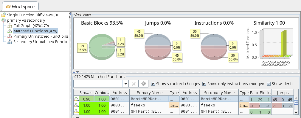
Example of BinDiff UI visualizing the QBinDiff generated result.BinDiff
QBinDiff as a library
QBinDiff was designed particularly to be used as a library for programmatic diffing. The previous example can be reproduced with the Python snippet below.
#!/bin/env python3
from qbindiff import Program, QBinDiff, LoaderType, Distance
from qbindiff.features import BBlockNb, CyclomaticComplexity, GraphDensity, DatName, MnemonicSimple

# Load binary disassembly using the binexport backend loader
print("[+] Loading primary: ./primary")
primary = Program(LoaderType.binexport, "./primary.BinExport")
print("[+] Loading secondary: ./secondary")
secondary = Program(LoaderType.binexport, "./secondary.BinExport")

# Initialize QBinDiff object
qbindiff = QBinDiff(
    primary,
    secondary,
    sparsity_ratio=0.7,
    distance=Distance.jaccard_strong,
)

# Register features
qbindiff.register_feature_extractor(BBlockNb, 2)
qbindiff.register_feature_extractor(CyclomaticComplexity, 1)
qbindiff.register_feature_extractor(GraphDensity, 1)
qbindiff.register_feature_extractor(DatName, 4)
qbindiff.register_feature_extractor(MnemonicSimple, 2)

print("[+] Initializing NAP")
qbindiff.process()

print("[+] Computing NAP")
qbindiff.compute_matching()

# Exporting the result to BinDiff format
qbindiff.export_to_bindiff("result.BinDiff")
After completing the diff, one can already play with the result without having to export it to a
BinDiff file format, in fact, it is possible to access the Mapping object
that contains the entire detailed mapping between functions with the similarity and confidence
scores.
from qbindiff import Mapping

def display_statistics(differ: QBinDiff, mapping: Mapping) -> None:
    nb_matches = mapping.nb_match
    similarity = mapping.similarity
    nb_squares = mapping.squares

    output = (
        f"Score: {similarity + nb_squares:.4f} | "
        f"Similarity: {similarity:.4f} | "
        f"Squares: {nb_squares:.0f} | "
        f"Nb matches: {nb_matches}\n"
    )
    output += "Node cover:  {:.3f}% / {:.3f}% | Edge cover:  {:.3f}% / {:.3f}%\n".format(
        100 * nb_matches / len(differ.primary_adj_matrix),
        100 * nb_matches / len(differ.secondary_adj_matrix),
        100 * nb_squares / differ.primary_adj_matrix.sum(),
        100 * nb_squares / differ.secondary_adj_matrix.sum(),
    )
    print(output)

# After computing the diff (qbindiff.compute_matching()) we can
# access the object qbindiff.mapping
display_statistics(qbindiff, qbindiff.mapping)
The result that we obtain should be pretty much the same as before.
Not a Binary? No Problem: Bioinformatics use-case
As shown above, QBinDiff is solving an optimization problem that goes beyond binary diffing. In fact, binary diffing is somehow just an instance of this problem. Different research fields, especially biology, also have this kind of problem.
We designed a low-level API that works on any kind of problem given the two core elements of the algorithm:
- A matrix representing the pairwise similarity between two objects in the problem domain.
- A generic graph where a node is the atomic object in the problem domain and edges represent relationships between objects.
In binary diffing, these base objects are functions, but they can be pages/profiles in social networks, or atoms in molecules analysis.
One important use case in bioinformatics is the alignment of protein-protein interaction (PPI) networks of different species8. A PPI network is a huge graph in which the nodes are proteins and edges represent interactions between them. A comparative study of these two graphs can reveal important insights that may help in disease analysis, drug design, understanding the biological systems of different species, and more.
In this example, we are going to analyze the PPI networks of Homo sapiens (human) and Mus musculus (mouse). These networks have been studied multiple times and as such are available in several open databases. In this case, we used the BioGRID public database, which archives and disseminates genetic and protein interaction data collected from over 70,000+ publications in primary literature.


Visualization of the PPI networks. On the left is displayed the Homo sapiens while on the right is the one of the Mus musculus. The colors help to identify graph communities
In order to provide a similarity matrix between the nodes (in this case the proteins) of the two graphs we can use the BLAST algorithm,9 that computes the similarity between two proteins by comparing their amino-acid sequences.
For the sake of clarity suppose that we already have Python objects representing the graphs and the similarity between the nodes.
import networkx

primary: networkx.Graph = load_graph(...)  # Homo sapiens PPI network
secondary: networkx.Graph = load_graph(...)  # Mus musculus PPI network
blast_scores: dict[tuple[str, str], float] = load_blast(...)  # BLAST similarity scores

print(f"Primary graph\n\tNodes: {len(primary)}  Edges: {primary.size()}")
print(f"Secondary graph\n\tNodes: {len(secondary)}  Edges: {secondary.size()}")
print(f"Size of similarity matrix {len(blast_scores)}")
Primary graph
    Nodes: 8932  Edges: 41158
Secondary graph
    Nodes: 1584  Edges: 2097
Size of similarity matrix 102667
Now that we have all the data we need, it's time to create a Differ instance and compute the
alignment of the two networks. Since we are working with undirected, unattributed graphs we can use
the GraphDiffer class from qbindiff.
To load the similarity matrix with our scores, we can register a Pass function. The pass mechanism
is used for refining the similarity matrix.
To populate the similarity matrix with the BLAST scores we can use the pass mechanism, a callback
system that is used for refining the similarity matrix at each pass. By default a GraphDiffer
instance will initialize the entire similarity matrix to 1, hence it's not leveraging similarity
information, so we can re-initialize it to 0 and then put the normalized similarity BLAST score.
from qbindiff import GraphDiffer, Program
from qbindiff.types import SimMatrix

def init_similarity_matrix(
    sim_matrix: SimMatrix,
    primary: Program,
    secondary: Program,
    primary_mapping: dict[Any, int],
    secondary_mapping: dict[Any, int],
    blast: dict[tuple[str, str], float],
) -> None:
    sim_matrix[:] = 0
    for (label1, label2), score in blast.items():
        sim_matrix[primary_mapping[label1], secondary_mapping[label2]] = score

    # Normalize
    sim_matrix /= sim_matrix.max()

# Create a differ instance
differ = GraphDiffer(primary, secondary, sparsity_ratio=0)

# Register a pass to populate the similarity matrix
differ.register_prepass(init_similarity_matrix, blast=blast_scores)

# Compute the diffing
mapping = differ.compute_matching()
print(f"Similarity: {mapping.similarity}  Normalized Similarity: {mapping.normalized_similarity}")
Similarity: 807.2150001265109 Normalized Similarity: 0.153521300898918
At this point it's easy to manipulate the Mapping object containing the alignment of the two PPI
networks.
The complete script as well with the dataset can be downloaded here.
Diffing portal
As part of our work on diffing, we tried to aggregate various resources and documentation about the various tools on a single web page: the diffing portal. It also contains in-depth explanations about the algorithm used by QBinDiff and other differs as well as tutorials and quick start guides, academic papers, and documentation about binary exporters and differs.
It can be reached at this link https://diffing.quarkslab.com/.
Conclusion
We open-sourced QBinDiff, an experimental tool that requires some know-how to get the most of it. However, it's a good platform for experimentation and more specific diffing tasks. Because of its implementation in Python, it never will be faster than Bindiff but it does not intend to :).
Multiple experiments are in the pipe especially to compare it against Diaphora3 and its features from the decompiled code. Also, more academic results are hopefully coming soon!
The goal of this post was to give an insight into QBinDiff's algorithm and how diffing can be applied beyond reverse-engineering. We are also eager to receive constructive feedbacks on our tools. To conclude, if you have other use cases where such approach can be useful, let us know!
-
Burkard, Rainer E. (Mar. 1984). Quadratic assignment problems. European Journal of Operational Research 15.3, pp 283-289. ↩
-
Bayati, Mohsen et al. (Dec. 2009). Algorithms for Large, Sparse Network Alignment Problems. Proceedings of the 2009 Ninth IEEE International Conference on Data Mining. ICDM '09 USA: IEEE Computer Society, pp, 705-710. ↩
-
Klau, Gunnar W. (Jan. 2009). A new graph-based method for pairwise global network alignment. BMC Bioinformatics 10.1, S59. ↩
-
Loeliger, H.-A. (Jan. 2004). An introduction to factor graphs. IEEE Signal Processing Magazine 21.1, pp. 28–41. ↩
-
Elie Mengin, Fabrice Rossi. Improved Algorithm for the Network Alignment Problem with Application to Binary Diffing. 25th International Conference on Knowledge Based and Intelligent information and Engineering Systems (KES2021), Aug 2021, Szczecin, Poland. pp.961-970. https://arxiv.org/abs/2112.15336v1 ↩
-
Elie Mengin, Fabrice Rossi. Binary Diffing as a Network Alignment Problem via Belief Propagation. 36th IEEE/ACM International Conference on Automated Software Engineering (ASE 2021), IEEE; ACM, Nov 2021, Melbourne, Australia. https://arxiv.org/abs/2112.15337 ↩
-
Titeca, Kevin; Lemmens, Irma; Tavernier, Jan; Eyckerman, Sven (29 June 2018). Discovering cellular protein‐protein interactions: Technological strategies and opportunities. Mass Spectrometry Reviews. 38 (1): 79–111. ↩
-
Stephen F. Altschul, Warren Gish, Webb Miller, Eugene W. Myers, and David J. Lipman. Basic Local Alignment Search Tool. Journal of Molecular Biology. 1990: 215(3) ↩