Author Le Maréchal
Category Software
Tags Ivy, NoSQL, MongoDB, Elasticsearch, development, software, 2015
A modest comparison between two ways of storing our unstructured data, from MongoDB to Elasticsearch.
Introduction
Historically, a significant part of QuarksLab's activity is composed of reverse engineering, malware analysis and offensive pentesting. But these occupations lead use to develop some nice tools we trust can be of a great use for any company willing to improve its own knowledge rather than externalize every security aspects.
Ivy is one of these tools, or, should we say, solution as it is now a mature project with industrial development process, automatic deployment, early clients and all the fancy stuff. Ivy is a massive network recon software, designed to detect potential flaws on large networks in the order of one to hundreds of millions of IP addresses (or more, depends on how much money your are willing to spend). The collector probes can perform many network operations, from trivial http-headers gathering to complex test of vulnerable services. "Who doesn't?" would you say - well, moreover, Ivy allows flexible custom plugins integration, to fit the most specific services, as long as it could be reached with an IP address (IPv4 for now; IPv6 is on its way).
Enough for the collector part; and we won't neither bother you with the neat dispatcher component. The whole thing for a software like Ivy is not as much to gather data as too give users access to a fast, precise, relevant data-mining engine. And here comes the database choice.
Environment
Equipment
Let's talk about equipment first. We don't want the Ivy frontend to run on top of expensive servers. That is way too easy - and cumbersome. We want the frontend to be running on portable, common computers: Raspberry Pi A... wait, kidding. We are talking about databases with million or billion entries, so let's try with a Intel Core 7 4700MQ processor, 8GB RAM with a regular SSD, which is a fair example (and also the exact specs the laptop used for most tests). We also have several users running Ivy into virtual machines, with 2 vCPU and 2GB RAM. When we need some more firepower, we have a server with an Intel Xeon E5-1620, 64GB RAM and RAID-0 SSDs. Nothing more: no heavy kickass server, no multinode cluster, no cloud service such as AWS.
Tools
The Ivy team is preferentially working with Python, so most (if not all) of the scripts in the following examples will be written with this language.
Also, global variables such as db or es are defined as:
db = pymongo.MongoClient()[<some_database>]
es = elasticsearch.Elasticsearch()
Where does Ivy come from
Ivy was born with MongoDB. The main problematic of the early versions of Ivy was to easily stored unstructured data. On every IP address scanned by Ivy, some ports could be open, some others not, sometimes none. Information could be collected, or not, plugin could match, gather incomplete data, raw data or structured data (what a mess...). In the end, the structure of one single IP address analysis can strongly differ from another one.
Unstructured database was a necessity from the beginning. And by that time, MongoDB sounded like the best choice: schemaless, BSON structured-documents, a solid Python client, good feelings from the community, a vast documentation, an intuitive CLI, promisingly powerful aggregations and some other nice gadgets (like the ObjectId).
The way we choose to store data on MongoDB was quite simple: every IP address of a scan is a document, belonging to a single collection. The most significant fields of an IP address are: which ports were opened, and which plugins gave a response back. These two fields could be quite complex.
For instance, here is a very basic IP address result:
{ "_id" : ObjectId("54c921e3902ed0377abffcab"),
  "country" : "US",
  "hostIpnum" : "1234567890",
  "tlds" : ["zetld.com"],
  "ports" : [{
      "service" : "http",
      "server" : "Microsoft IIS",
      "version" : "",
      "port" : {
          "value" : 443,
          "protocol" : "tcp"
      }}],
  "pluginResults" : {
      "sc:nse:http-headers" : [{
          "relatedPorts" : [{
              "value" : 443,
              "protocol" : "tcp"
          }],
          "data" : {
              "outputRaw" : "\n  Content-Length: 3151  \n  \n  (Request type: GET)\n"
          }}],
      "sc:nse:sslv2" : [{
          "relatedPorts" : [{
              "value" : 443,
              "protocol" : "tcp"
          }],
          "data" : {
              "outputRaw" : "\n  SSLv2 supported\n    SSL2_RC4_128_WITH_MD5\n    SSL2_DES_192_EDE3_CBC_WITH_MD5"
          }}]}
}
MongoDB has no problem storing or managing such document.
We started then developing two more interesting features: filters and aggregations.
Filters exactly means the word. Filtering irrelevant IP addresses, whatever the discriminant factor, is an essential key for efficiently dive into the results. A very simple filter could be display only the IP addresses with at least 4 opened ports.
Aggregations are meant to quickly highlight a particular point of view on a scan. Ivy does not really fit one to one IP address analysis. Its goal is to enlighten an entire network. Computed data like the distribution of the number of open ports, the sorting of most services discovered on the network, or simply the different countries the IP addresses belong to are useful information users must have immediate access and at will. Of course, the aggregations must always fit the current filters. For instance, display the distribution of services name with their version over all the IP addresses is an aggregation.
Inferno - The twilight of MongoDB
Apocalypse
All these pretty features went smooth and nice on our basic example sets. Our testing process was still young and we were lacking a whole platform with a life-sized sample to stress our developments, so we just didn't saw what was coming.
We were accepted to deliver an introduction to Ivy during the 2014 Hack In The Box conference in Malaysia. For the event, we migrated a previous dense scan we had on this country. The country wasn't that big -7 million IP addresses, we had already done far bigger-, but we tested many ports and many plugins, and the results were fat. We prepared a VM for the demonstration, and then tested it.
The performances were so bad the HTTP server was just throwing timeout errors, leaving the UI empty and cold like Scottish moors during winter.
We measured the aggregations were taking between 30 and 40 seconds each. Knowing we designed the front page of a scan to host 4 basic aggregations, and the system was stuck for several minutes without being able to accept any other request accessing the database.
How did we manage to improve the performances? Well, has always when deadlines come close: with dirty hacks. We set up a really non-subtle cache mechanism, split the IP addresses single collection into a dedicated IP addresses collection for each scan, filled them with indexes, and finally pushed the VM up to 6GB RAM.
Our Ivy VM didn't mess us up during the conference, but it was now clear we got some nasty performance issues in our system.
Ivy has not been designed to be completely enslaved to MongoDB. In fact, the data abstraction was strong enough for us to change our database quite easily. Of course, some technical debts were to be removed, but the most part of the code - the filters - was build using a custom IR (Intermediate Representation), allowing us to switch database 'only' by implementing an IR_to_new_db translation class.
But as complete newbies of MongoDB, we thought we were just doing wrong with it, and so we took some time testing and stressing our system to improve our performances without changing our database choice.
Fixing the cripple
Dedicated collection
Dedicated IP addresses collections for each scan was a poor fix we eventually properly integrated into Ivy. The idea was not really to improve speed on large scans, but rather to allow fast exploration in small and medium scans without being slowed down by the results of the bigger ones.
Pre-calculated figures
The aggregations on Ivy were dynamic, because they are calculated accordingly to the current filter. We pre-calculate the aggregations for the empty filter, which is the default state, so that results are immediately displayed.
The current issue with this system is the scary time response gap users experiment as soon as they apply a filter, as aggregations go to static pre-calculated immediate figures to live-calculated slow results, while the volume of data on which the aggregations are calculated on is smaller.
Indexes
We realized some indexes were just not efficient at all. Indexes on 'root leaves' are powerful. But our most interesting information are stored deeper on documents.
For instance, let's talk about filtering on the port number. A really common request we want to do looks like {"ports.port.value": 53}. That really isn't complex at all. But applied on a 22 million IP addresses scan on a laptop, the results do not smell simplicity:
168 seconds without index,
121 seconds with a single index,
116 seconds with a sparse index (a sparse index ignores documents without the indexed field).
The scariest figure here is not the unacceptable response time. It is the tiny ~1.39 ratio (~1.46 with sparse index) between a request without any index, and a request with an index. Just to compare, a request on a 'root leaf' like "hostIpnum" (request is {"hostIpnum": 1234567890}), we have:
323.808 seconds without index,
0.148 seconds with a single index,
0.103 seconds with a sparse index (with the fact that a document without "hostIpnum" field can't even exist...)
... meaning a ~2186.68 ratio (~3151.69 with sparse) between the index and none, clearly a much more efficient index.
We initially thought that list-typed fields, just like our "ports" field, completely destroyed MongoDB index performances. As two of the most important information parts gathered by Ivy, ports and plugins, were stored in list, we thus tried with a slightly different format, without list, and so the performances should be better. We try to switch the representation of the ports, from the old:
{"ports": [ {"port": {"value": <value1>
                      "protocol": <protocol1>},
             "service": <service1>,
             "version": <version1> },
             {"port": {"value": <value2>
                      "protocol": <protocol2>},
             "service": <service2>,
             "version": <version2> },
             ...],
...}
... to :
{"ports": {<protocol1>: {<port1>: {"service": <service1>,
                                   "version": <version1>},
           <protocol2>: {<port2>: {"service": <service2>,
                                   "version": <version2>},
           ...},
 ...}
... so the request wasn't {"ports.port.value": 80} anymore, but something like {"ports.tcp.80": {"$exists" 1}}.
This solution is not viable, because of some IP addresses with lots of opened ports (more than 20, which is far to be rare). Because the index is applied either on "ports" or "ports.<protocol>", the containing BSON documents could exceed the 1024 bytes index key limit, and so document insertion (or index construction) could fail. Let's say we play the game and put an index on "ports.tcp.80" (meaning that if it works, we should put an index on the 65,535 possible ports for both tcp and udp protocols). The measures (with MongoDB explain method) on a 566,371 IP addresses collection are:
67 seconds without index,
108 seconds with a single index,
58 seconds with a sparse index.
The numbers don't need comment to disqualify this idea.
An inelegant workaround we implemented was to calculate basic information ("nbOpenedPorts" <int> and "hasPluginResults" <bool>) on each ports and plugins information, stored as root leaves on our IP address documents, with single indexes, allowing Ivy to inject more conditions on its requests (for instance {"nbOpenedPorts": {"$gt": 0}, "ports.port.value": 53}). As the explain underlines, MongoDB always uses these new efficient indexes to perform its requests, rather than the older and slower ones. Performances on a 22 million documents collection (on our strongest computer) are:
23.6267 seconds with {"ports.port.value": 53}
1.7939 seconds with {"nbOpenedPorts" : {$gt: 0}, "ports.port.value": 53}
... which is the difference between a user ragequit and a "not-so-smooth-but-acceptable" user experience.
But this strategy has its limits, as MongoDB can't take advantage of several single indexes at the same time. In fact, MongoDB throws the requests on every indexes independently (and also throws an index-free request), and awaits for the fastest to achieve, then terminates the others. So the most narrowed request can't be faster than a vague request on the most efficient index.
Adding compound indexes couldn't be considered, because the Ivy filter and aggregation engine is just to complex to anticipate every possibilities and it would be absurd to create compound indexes to fit every request. And even if we were willing to do so, MongoDB only allows 64 indexes max per collection. It is an annoying limit for our ambition to play with data in any possible way. As far as we know, this limit can't be changed through the configuration file.
Purgatorio - Still feeling a little tense in here
Time is everything
With these modifications and a few other tricks, we had a fairly usable system, able to manage 5-10 million IP addresses scans on a laptop, and up to 25-30 million IP addresses scans on our server. That was still a severe disappointment compared to our initial ambitions.
The aggregations were certainly our greatest deception. As our wishes with Ivy was to deliver the most freedom for user to set up their own metrics, we were excited to develop a very flexible aggregation engine inside the software. Our optimizations were reasonable for our current engine - huge freedom for filters, and simple and predetermined aggregations displayed with acceptable time. But it was obvious that we couldn't let users control the aggregation because of the poor performances.
We could have add more hard-coded optimized aggregations, the distribution of SSL public key sizes for instance. But that would only have been a camouflage with the guarantee that one day or another, the metrics we defined will not fulfill the need of a user.
Space and dark matters
Moreover, we weren't very comfortable with some of MongoDB's "largesses", especially when it came to administrate or manage our frontends.
MongoDB clearly doesn't care about space. At all. Disabling data file preallocation or using small files won't stop MongoDB to eventually devour our space disk and RAM.
First of all, MongoDB deliberately keeps large unused space ranges between documents while inserting them, in order to efficiently sort later insertions. The indexes also take a very significant part of the whole space disk. For instance, on a newly created (so hopefully with minimum fragmentation losses) collection with 9 indexes (including the default "_id" index), we have:
size of the BSON file used for the collection restoration: ~2.77GB
db.<collection>.count(): 6,357,427 documents
db.<collection>.dataSize(): ~4.08GB
db.<collection>.storageSize(): ~4.47GB
db.<collection>.totalIndexSize(): ~1.20GB
db.<collection>.totalSize(): ~5.67GB
The disk space is not really an issue here (for now...), but the indexes should be in RAM to be efficient. Knowing that on a final Ivy frontend, a collection like this is considered average and has many other siblings, we began to sweat for our performances.
MongoDB also has a wild tendency to fragmentation, both on disk and RAM. Using update and remove has dangerous incidences on collections, and so does storing documents with various sizes (which really is the case with Ivy, as some IP addresses could be totally mute and others very talkative). The result is that a collection reduced to a few thousands documents after counting millions won't free that much space - in fact, it won't free any space at all.
The technical choices explaining this space consumption are understandable, but it doesn't take out the fact that it is painful in some situations we often dealt with:
manipulating VM .ova (compressing, uploading, downlading, etc.),
database dumps / restoration (still mongodump and mongorestore are very handy tools),
trying to reduce the database space disk (quite ironic uh? the db.repairDatabase command, designed to shrink a database, needs enough place to duplicate this whole database. "- Hey, I need space, let's shrink a db! - Hope you got a few hundred free gigabytes for that, buddy...").
Well...
We ended up at a point where we still had a few points we guessed we could gain performances on. But the changes needed were deep and costly, for unpredictable profits. So we provisioned time to test other technologies, among which was Elasticsearch.
Paradisio? - The dawn of Elasticsearch
There no such thing as a trivial and direct skills comparison table between MongoDB and Elasticsearch. It can't be. The two systems do not seek achieving the same goals, and they don't treat data the same way.
Let's hide behind the words: MongoDB is a database whereas Elasticsearch is a search engine. It really comes to sense when manipulating these two systems: whereas MongoDB is all about flexibility with data, Elasticsearch has a bit more cautious and ordered approach.
First of all, a quick overview of Elasticsearch. In fact, Elasticsearch is - rudely speaking - a wrapper around the text search engine library Lucene. Schematically, Lucene manage low-level operation, as indexing and data storage, while Elasticsearch brings some data abstraction levels to fit JSON possibilities, an HTTP REST API and eases a lot the constitution of clusters.
From now, as we don't talk about other search engine like Solr, or Lucene-only exploitation, and as Elasticsearch can hardly work without Lucene, we won't make any formal difference between the two and will only talk about Elasticsearch as a whole.
Poking the bear
The very first move we made while testing Elasticsearch was to at least reproduce the same behavior we had with MongoDB.
Filters
N.B: We are talking about filters in the Ivy way. The Elasticsearch's request system deals with other filter and query notions we won't bother with, as they are not in this article scope.
The filters were easy to replicate, just the time to assimilate the Elasticsearch request system and to find the equivalences. Though, we already managed to point out some minor improvements on the logic of Elasticsearch requests compared to the MongoDB one.
For instance, we always had trouble with the MongoDB $not operator, to negate a pre-defined filter. Let's take for instance the filter:
{"nbOpenedPorts": {$gt: 4},
 "ports.port.value": 80}
$not can't be a top level operator, meaning we can't ask for:
{$not: {
  "nbOpenedPorts": {$gt: 4},
  "ports.port.value": 80
}
... we need to "propagate" the $not to all the leaves of the filter.
Moreover, $not needs to be applied to an expression, either a regular expression or a another operator expression, so the negation of {"ports.port.value": 80} can't directly use $not but needs the $ne operator.
So we need a pass that would propagate the not operator through the IR, invert every operator one by one, apply the De Morgan laws, and replace $not by $ne when needed. Finally, the negation will be:
{ $or: [
  {"nbOpenedPorts": {$not: {$gt: 4}}},
  {"ports.port.value": {$ne: 80}}
]}
In Elasticsearch, operators are used in a very homogeneous and logical way that prevent that sort of trickery.
The original request equivalence is:
{"filter": {"and": [
  {"term":
    {"ports.port.value": 80}},
  {"range":
    {"nbOpenedPorts": {"gt": 4}}}
]}}
... which is, yes, fatter but has the advantage to be completely unambiguous.
To negate this request, the not operator could easily be included on top like this:
{"filter": {"not": {"and": [
  {"term":
    {"ports.port.value": 80}},
  {"range":
    {"nbOpenedPorts": {"gt": 4}}}
]}}}
... straight to the point.
Meanwhile, we glanced the time taken by these requests. On a laptop, with a filter on a 6,357,427 documents collection, we counted the documents fitting the previous requests:
14.649 seconds for MongoDB,
0.715 seconds for Elasticsearch,
... meaning a ~20.5 ratio at best between MongoDB and Elasticsearch in favor of the last one.
Aggregations
As we said below, the Elasticsearch request system is very homogeneous, and it becomes clear when dealing with aggregations.
MongoDB has a dedicated aggregation pipeline, defined through the stages [{"$match": <query>}, {"$group": <agg>}, {"$sort": <sort>}, ...].
Elasticsearch aggregations are totally integrated into the requests, and even if the request body is generally bigger than a MongoDB pipeline, it feels way clearer.
Let's take the example of the very simple "by country" aggregations. We want the number of IP addresses for every country in the scan.
The MongoDB pipeline answering this is:
[{"$group": {"_id": "$country", "total": {"$sum": 1}}}, # Sum of IP addresses by "country"
 {"$sort": {"_id": 1}}]                                 # Sort on the country names
And the Elasticsearch one is:
{"aggs": {<agg_name>:
           {"terms": {"field": "country",          # Aggregation on field "country"
                       "size": 0                   # Return every buckets
                       "order": {"_term": "asc"}}  # Sort on the country names
}}
Again, the Elasticsearch performances relatively to MongoDB are astonishing. On the same laptop, and the same collection, we measured:
42.116 seconds for MongoDB (first try),
3.799 seconds for MongoDB (second try, the first aggregate "warmed up" the RAM),
0.902 seconds for Elasticsearch (first try).
... meaning a ~46.7 ratio at first try (~4.2 at second try) between MongoDB and Elasticsearch in favor of the last one.
We ain't goin' out like that
One aspect where Elasticsearch strongly differs from MongoDB is that it is not schema-less. It is possible to index document without any more information than the data alone, but the engine automatically maps the fields. When indexing a document, Elasticsearch defines a default mapping for it. Once it's defined, it is not possible (unlike MongoDB) to index another document with the same type but a different format (with a string in a former int field for instance).
And here comes the mapping, the concept that maybe explains the much better results of Elasticsearch against MongoDB for filters and aggregations, and could just as much giving a useful meaning to our data as destroying our application by returning false results.
String analysis
For instance, by default, Elasticsearch analyzes the string fields so that a field with "Foo&Bar-3" will be schematically tokenized into "foo", "bar", "3". This division helps sorting the text in an inverted index (used by Lucene), and the word normalisation (lowercasing in this case) improve research performances. Elasticsearch offers several different analyzers, it is even possible to define one.
But in our case, we want the exact matching value. The string field analysis was returning false data for our filters and aggregations. For instance, when aggregating on ports.port.server, services like ccproxy-ftp wouldn't showed up, they were be counted like one ccproxy and one ftp, leading to a totally wrong result.
Fortunately, it is possible to deactivate this analysis in the mapping of the document, by redefining the default mapping from:
{<field_name>: {"type": "string"}}
to:
{<field_name>: {"type": "string":
                "index": "not_analyzed"}}
Or, if we want both the field to be analyzed and being accessible as not analyzed:
{<field_name>: {"type": "string",
                "fields": {<subfield_name>: {"type": "string",
                                             "index": "not_analyzed"}
}}
... so that the analyzed field is accessible on regular field <field_name>, and the non-analyzed field on <field_name>.<subfield_name>.
Document flattening
The string analysis could be somehow disturbing the first hours with Elasticsearch (particularly the first aggregations with freaky wrong results), but it is no big deal.
Elasticsearch default mapping has deeper strong effect, such as the array flattening.
Our data model stored opened ports of an IP address as a ports list, like:
{"ports": [{"port": {"value": 80,
                     "protocol": "tcp"},
            "server": "thttpd",
            "service": "http",
            "version": "2.25b 29dec2003"},
           {"port": {"value": 5000,
                     "protocol": "tcp"},
            "server": "",
            "service": "upnp",
            "version": ""},
            ...
]}
By default, Elasticsearch does not interpret the documents in the ports list as a set of independent documents, but flatten them in something like:
{"ports.port.value": ["80", "5000"],
 "ports.server": ["thttpd"],
 "ports.service": ["http", "upnp"],
 "ports.version": ["2.25b 29dec2003"] # let's suppose we deactivated the string analyzing here
}
Again, it is clear how this ordering eases the inverted index of Lucene. This feature is really powerful for text search, as splitting a sentence in words enable to sort documents by proximity to the request, and helps returning more relevant searches (just like Google offers different words or sentences when searching). The Elasticsearch more like this query is a very obvious example of that.
However in our case, it is a misleading feature. Elasticsearch would return the previous example as a rightful match if we searched for a document with {"server": "thttpd", "service": "upnp"}. And an aggregation on service versions would return a service upnup with version 2.25b 29dec2003, which does not exist.
The solution is still in the mapping. The nested type explicitly keeps nested documents separated. Declaring a field as nested is not complex - just add "type": "nested" in the field mapping - but including nested fields in queries significantly changes them. A request on ports.port.value = 80 previously looked like:
{"filter": {"term": {"ports.port.value": 80}}}
now becomes:
{"filter": {"nested": {
      "path": "ports",   # "ports" is the nested document here
      "filter": {"term": {"ports.port.value": 80}}
}}}
And the bigger the request goes, the lesser we can quickly understand it. But hey! that's why computers are made for (these requests are created from our filtering IR).
Take a look under the hood
Inserting documents
These mapping configurations underline a dark (but necessary) side of Elasticsearch: mapping can't be modified afterwards. It must be redefined elsewhere and all the data migrated from the previous type to the newer.
This constraint was the pretext to compare Elasticsearch insertion mechanisms with MongoDB's. Both of them has bulk method to insert loads of documents.
A pymongo bulk insertion could be like:
def mongo_bulk(size):
  start = datetime.datetime.now()
  count = 0
  bulk = db.<collection>.initialize_unordered_bulk_op()    # Initializing the bulk. We don't need any order
                                                           # for pure insertion
  bulk.find({}).remove()                                   # Cleaning the output <collection>
  for doc in document_list_or_generator_or_whatever():
    count += 1
    bulk.insert(doc)
    if not count % size:                                   # A good value for 'size' could be 10k docs
      bulk.execute()
      bulk = db.<collection>.initialize_unordered_bulk_op()
      count = 0
  bulk.execute()
  return datetime.datetime.now() - start
... while an elasticsearch implementation would be more like:
def es_bulk(size):
  start = datetime.datetime.now()
  insert = list()
  for doc in document_list_or_generator_or_whatever():
    insert.append({"index": {"_index": <index>,        # The metadata explaining how to treat the following
                             "_type": <doc_type>}})    # document. We simply index it here
    insert.append(doc)                                 # The document to be indexed
    if not len(insert) % size*2:                       # Due to metadata (see below), the list length is twice
                                                       # the number of documents to insert
      es.bulk(insert)
      insert = list()
  es.bulk(insert)
  return datetime.datetime.now() - start
The two Bulk APIs are very similar, with the same methods (insert, update, remove, etc.) and the same logic (possibility to update document with scripts such as incrementing an int, and so on). On a laptop, for an insertion of 6,357,427 documents (provided by the same document_list_or_generator_or_whatever), we had:
MongoDB (loads of 10k documents): 522 sec -> ~12,159 documents/second
Elasticsearch (loads of 10k documents, no mapping): 600 sec -> ~10,597 documents/second
Elasticsearch (loads of 10k documents, custom mapping): 626 sec -> ~10,161 documents/second
These are rather similar results. MongoDB is ~1.15 faster than Elasticsearch with a default-mapped index, and ~1.20 faster than a custom-mapped one.
Scrolling data sets
MongoDB's useful limit and skip methods allow to travel along our data. Elasticsearch has a slightly different functioning, as we must explicitly use a scroll method to do so.
The pymongo code will be:
def mongo_scroll(chunk):
    results = list()
    for a in range(0, int(db.<collection>.count()/chunk)+1):
        start = datetime.now()
        list(db.<collection>.find().skip(a*chunk).limit(chunk)) # 'list' to force the cursor to get data
        results.append(datetime.now()-start)
    return results
And the elasticsearch:
def es_scroll(chunk):
    results = list()
    scroll = es.search(<index>, <doc_type>, size=chunk, scroll="1m")
    for a in range(0, int(es.count(<index>, <doc_type>)["count"]/chunk)+1):
        start = datetime.now()
        scroll = es.scroll(scroll["_scroll_id"], scroll="1m")
        results.append(datetime.now()-start)
    return results
The following figures illustrate the results with chunks of 100k documents, on 23+ millions documents.
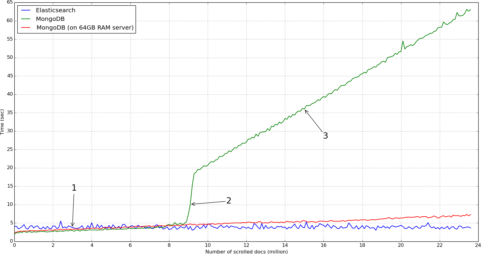
MongoDB clearly beats the first chunks, but has a tendency to slow down, unlike Elasticsearch which is very constant in its responses.
This sudden and huge gap on the MongoDB time response at ~9 million IP addresses seems to be that the cache switches from RAM reads to disk reads. We noticed that read IOs went from ~600/s to ~8,000/s, the read rate on disk went from ~20M/s to ~150M/s and page faults went from peaks at ~4,000/s to an average level at ~8,000/s.
Measures on our server with 64GB supports this analysis: the system is never out of RAM and thus the response time continues its slow rise without any sudden ramp.
Elasticsearch still sticks to ~4s of response time, MongoDB on 64GB RAM server peacefully rises, while MongoDB on laptop has a troubling slope (with response delay longer than a minute in the end).
A closer look of the first chunks (before the ramp):
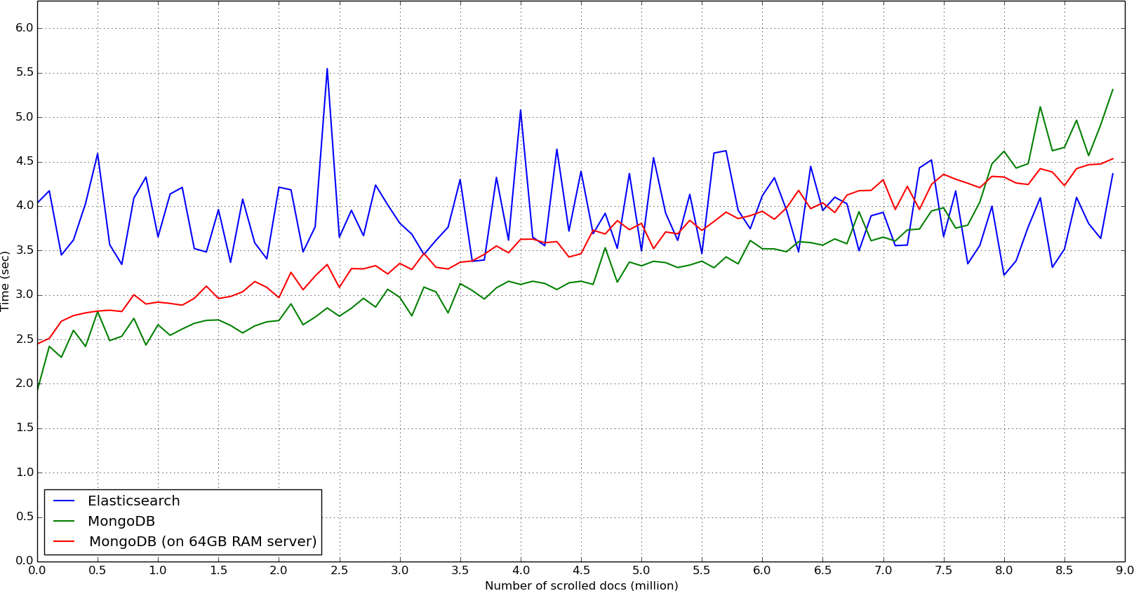
In fact, MongoDB does not have a real scrolling method like the Elasticsearch scroll, whose purpose is, at each call, to gather the following documents for the next call. On the contrary, the MongoDB find + skip + limit mechanism crossed the collection each time for the cursor to point on the first asked document. This could lead to severe performances issues when coupled with the sort method, which is greatly time-consuming, as the collection will be sorted at each call.
In any case, a 23 million documents data set is certainly a serious set, but yet not an extraordinary one. This highlights how MongoDB suits our small models, but has difficulties matching bigger needs when used on regular Ivy environment.
N.B.: MongoDB leaves the memory management to the operating system, so we can't blame it directly, but still, the curve is depressing...
Off topic: comparing disk space
As we won't be able elsewhere to directly compare the size taken by MongoDB or Elasticsearch, on this 23 million document data set, MongoDB disk space (without any index) was 26GB, whereas Elasticsearch only took 14GB. We don't know for sure if "Elasticsearch takes less space than MongoDB" is a general rule, but it just is with our document sets.
Aggregations - the new deal
The insertion and scrolling performances were not that impressive, and MongoDB has still arguments to fight with. But if we go back to basis, the very reason that started to make us question about MongoDB was the aggregations issue. In Ivy, the preceding mechanisms are mainly used during administration or migration tasks, without real time constraints. Unlike the aggregations which are used by the user who needs a responsive UI.
Performances on aggregation are consequently the judge between the two engines.
Enough talking
To compare the aggregation performances, we select five different data sets, from little ~29K documents set to an average ~29M documents set.
Two aggregations were tested: the very simple "by country" aggregation we already talked about above, and a more complex called "by server version".
This last aggregation calculates the distribution of couples of (<server name>, <server_version>) over the IP addresses. It is very useful to display an overview of, say, the IP addresses hosting a deprecated or vulnerable service. This aggregation is usually the one that causes real problems to MongoDB as soon as data sets reach 10-15 million of documents.
The MongoDB pipeline for the "by server version" aggregation is:
[{"$unwind": "$ports"},
 {"$match": {"ports.server": {"$exists": True, "$ne": ""}}},
 {"$group": {"_id": {"server": "$ports.server", "version": "$ports.version"},
             "total": {"$sum": 1}}},
 {"$sort": {"total": -1}}]
The Elasticsearch aggregation is:
{"aggs": {"a1":
    {"nested": {"path": "ports"},
     "aggs": {"a2":
         {"terms": {"field": "ports.server", "size": 0},       # First aggregation on 'ports.server'
          "aggs": {"a3":
              {"terms": {"field": "ports.version", "size": 0}} # ... and for each, aggregation on 'ports.version'
         }}}}},
 "filter": {"nested":
     {"path": "ports",
      "filter": {"bool": {"must": {"exists": {"field": "ports.server"}}}}
}}}
Using Elasticsearch without mapping, this aggregation would certainly miserably crash (meaning would return badly false results): "2.2.8" Apache version would be aggregated with "Allegro RomPager" server, version "4.51 UPnP/1.0" would be splat in meaningless tokens, etc.
But let's consider this mapping done and directly go to the results.
"by country" aggregation results
| Document number | MongoDB (sec) | Elasticsearch (sec) | Ratio (MongoDB/Elasticsearch) |
|---|---|---|---|
| 29,103,278 | 19.435 | 0.758 | 25.647 |
| 24,504,269 | 16.795 | 0.774 | 21.693 |
| 4,213,248 | 3.972 | 0.133 | 29.891 |
| 336,832 | 0.299 | 0.056 | 5.325 |
| 28,672 | 0.024 | 0.005 | 4.863 |
"by server version" aggregation results
| Document number | MongoDB (sec) | Elasticsearch (sec) | Ratio (MongoDB/Elasticsearch) |
|---|---|---|---|
| 29,103,278 | 106.539 | 2.736 | 38.943 |
| 24,504,269 | 102.604 | 1.866 | 54.983 |
| 4,213,248 | 13.752 | 0.224 | 61.344 |
| 336,832 | 1.286 | 0.050 | 25.750 |
| 28,672 | 0.103 | 0.008 | 13.620 |
Conclusion
These results highlight that MongoDB really isn't a good choice for our needs. Like we rambled from the beginning of this article: aggregation performances are the key for a software like Ivy, and these tables simply kill the debate in favor of Elasticsearch.
There is no such thing as a free lunch
Let's temper a bit about Elasticsearch. It is not the ultimate solution to save kitties, and has its defaults:
The mapping constraints force us to be very careful about Elasticsearch results when integrating new features, as they may be incorrect due to internal ordering as described above. But there is also a big chance that this is why Elasticsearch performs better for our queries.
Elasticsearch does not solve older problems we already had with MongoDB, such as the issue to store 128 bits integers and to do real calculations on them (helloo IPv6!).
Not a real performance/storage issue but still, managing an Elasticsearch node is not as simple as managing a MongoDB base, as we haven't found equivalent of tools like mongorestore or mongodump.
Though, and even if MongoDB has better bulk insertion performances and is more flexible, Elasticsearch is really a more promising engine for our needs, and Ivy is now migrating on it.